14. ANCOVA

Author

Affiliation

Johnny van Doorn

University of Amsterdam

Published

October 7, 2025

In this lecture we aim to:

Introduce ANCOVA
Implications of multiple predictors
Show ANCOVA in JASP

Reading: Chapter 12

ANCOVA

Determine main effect while accounting for covariate

1 dependent variable
1 or more independent variables
1 or more covariates

A covariate is a variable that can influence the DV. By adding a covariate, we reduce error/residual in the model.

Assumptions

Same as ANOVA
Independence of the covariate and treatment effect §12.5.1.
- No difference on ANOVA with covar and independent variable
- Matching experimental groups on the covariate
Homogeneity of regression slopes §12.5.2.
- Visual: scatterplot dep var * covar per condition
- Testing: interaction indep. var * covar

Independence of the covariate and treatment effect (Fig 12.2)

Data example

We want to test the difference in extraversion but want to also account for openness to experience.

Dependent variable: Extraversion
Independent variabele: Nationality (#groups \(= k = 3\))
- Dutch
- German
- Belgian
Covariate: Openness to experience

Define the model

\[{extraversion} = {model} + {error}\]

\({model} = {independent} + {covariate}\) \(\color{white}{model} = {nationality} + {openness}\)

\(\color{white}{model}\)

Linear model with \(k-1\) dummy variables:

\[\hat{y} = b_0 + b_1 {dummy}_1 + b_2 {dummy}_2 + b_3 covar\]

The data

Dummies

Observed group means

aggregate(extraversion ~ nationality, data, mean)

  nationality extraversion
1       Dutch     39.68286
2      German     40.86714
3     Belgian     37.60000

Model fit without covariate

What are the beta coefficients when we fit a model that only has nationality as a predictor variable?

fit.group <- lm(extraversion ~ nationality, data); fit.group$coefficients

       (Intercept)  nationalityGerman nationalityBelgian 
         39.682857           1.184286          -2.082857

\(\beta_{0} = 39.68\)
\(\beta_{German} = 1.18\)
- Prediction for German: 39.68 + 1.18 = 40.86
\(\beta_{Belgian} = -2.08\)
- Prediction for Belgian: 39.68 + -2.08 = 37.6

Model fit with only covariate

What are the beta coefficients when we fit a model that only has openness as predictor variable?

fit.covar <- lm(extraversion ~ openness, data); fit.covar$coefficients

(Intercept)    openness 
  24.993473    1.799697

\(\beta_{0} = 24.99\)

\(\beta_{Open} = 1.8\)

Model fit with all predictor variables (factor + covariate)

What are the beta coefficients when we fit the full model (i.e., with both predictor variables)?

fit <- lm(extraversion ~  nationality + openness, data); fit$coefficients

       (Intercept)  nationalityGerman nationalityBelgian           openness 
        25.9029405         -0.1220751         -2.7012528          1.8036540

\(\beta_{Dutch} = 25.9\)

\(\beta_{German} = -0.12\)

\(\beta_{Belgian} = -2.7\)

\(\beta_{Open} = 1.8\)

Predictions of the full model

For a German with a score of 8 on Openness:

fit <- lm(extraversion ~ nationality + openness, data); fit$coefficients

       (Intercept)  nationalityGerman nationalityBelgian           openness 
        25.9029405         -0.1220751         -2.7012528          1.8036540

\(\beta_{0} = 25.9\)
\(\beta_{German} = -0.12\)
\(\beta_{Open} = 1.8\)
- Prediction for German: 25.9 + -0.12 + 8 * 1.8 = 40.21

How about a Belgian with 6 Openness?

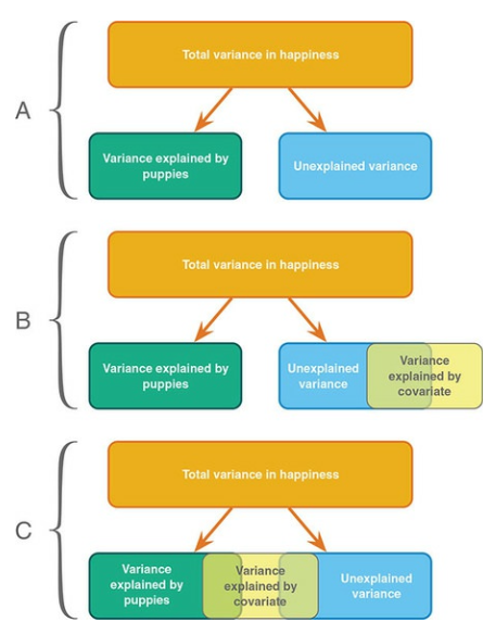
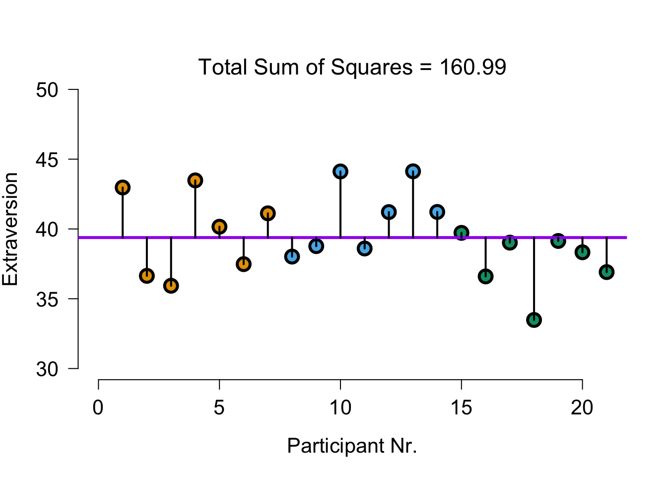
Total variance visual

Explained by group model

The model that predicts only using group means:

\(\hat{y} = b_0 + b_1 {dummy}_1 + b_2 {dummy}_2\)

\(\hat{y} = 39.68 + 1.18 \times {dummy}_1 + -2.08 \times {dummy}_2\)

Explained by group model - visual

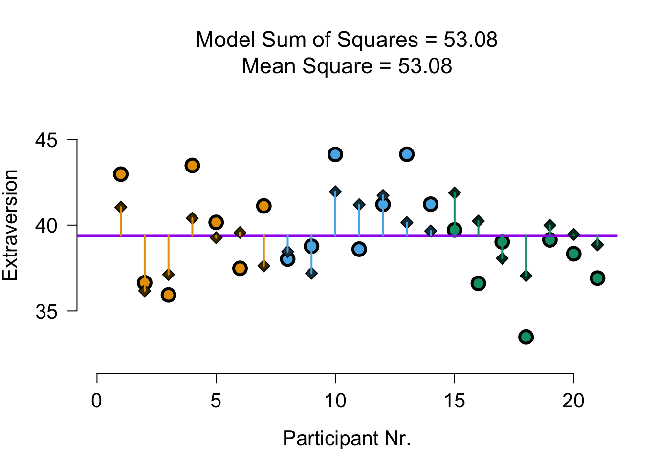
Explained by covariate model

The model that predicts only using openness:

\(\hat{y} = b_0 + b_3 covar\)

\(\hat{y} = 24.99 + 1.8 \times {Openness}\)

Explained by covariate model - visual

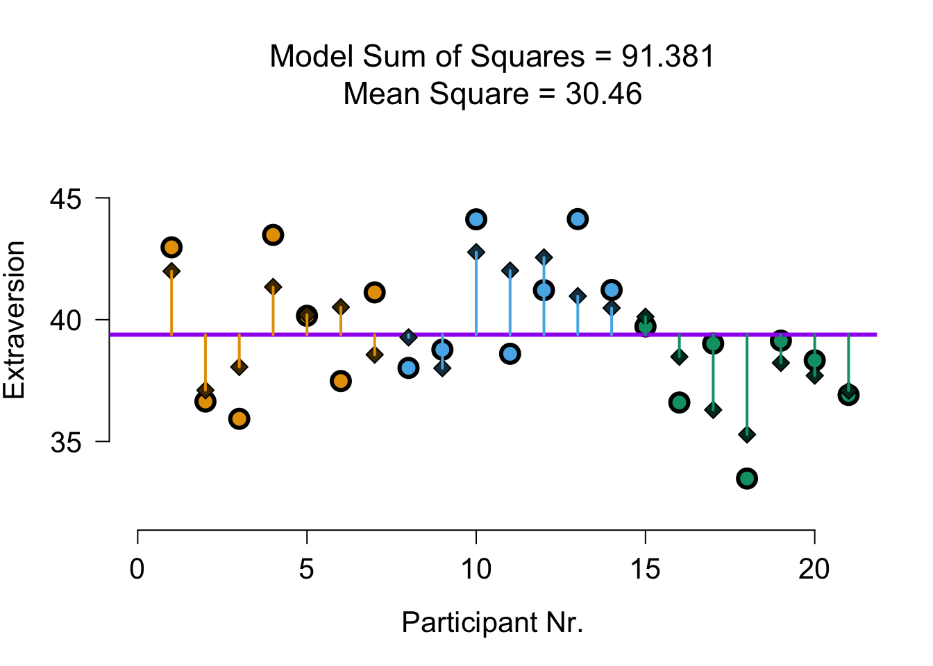
Explained by full model

The model that predicts with group and covariate:

\(\hat{y} = b_0 + b_1 {dummy}_1 + b_2 {dummy}_2 + b_3 covar\)

\(\hat{y} = 25.9 + -0.12 \times {dummy}_1 + -2.7 \times {dummy}_2 + 1.8 \times {Openness}\)

Explained by full model - visual

Unexplained variance (group and cov)

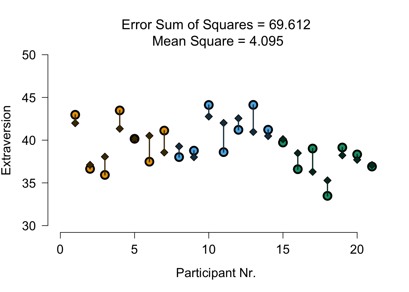
Divide model sum of squares

Model SS of full model:

SS.model

[1] 91.38149

To see what is explained by group, we subtract the Model SS of the covariate model:

SS.group <- SS.model - SS.model.covar; SS.group ## SS.group corrected for covar

[1] 32.58198

To see what is explained by covariate, we subtract the Model SS of the group model:

SS.covar <- SS.model - SS.model.group; SS.covar ## SS.covar corrected for group

[1] 53.07971

F-ratio

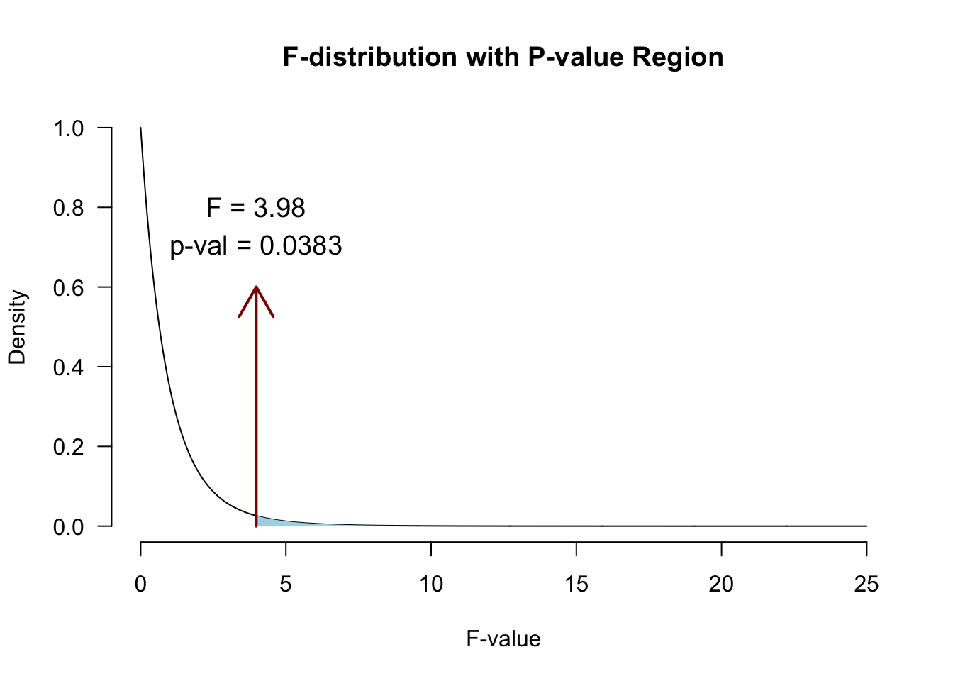
\(MS_{model-group} = \frac{32.582}{2} = 16.291\)

\(F = \frac{{MS}_{model}}{{MS}_{error}} = \frac{{SIGNAL}}{{NOISE}} = \frac{16.291}{4.095} = 3.98\)

\(P\)-value

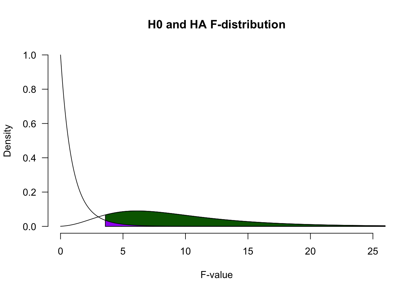
Alpha & Power

Power becomes quite abstract when we increase the complexity (i.e., number of predictors) of our models. We can make an F-distribution that symbolizes the alternative distribution by shifting the distribution more to the right (although the interpretability becomes pretty murky..)

Adjusted/marginal means

Marginal means are estimated group means, while keeping the covariate equal across the groups

What are extraversion averages in each group, if they would all score the same on openness?

Adjusted/marginal means

Adjusted:

  nationality mean.adj
1       Dutch 40.32444
2      German 40.20237
3     Belgian 37.62319

Observed:

  nationality extraversion
1       Dutch     39.68286
2      German     40.86714
3     Belgian     37.60000

JASP

Closing

Recap

We can add a continuous predictor to the ANOVA model, to reduce the overall model error
With multiple predictors, we need to check:
- Whether there is an interaction effect
- Whether the predictors are associated

Recommended Exercises

Exercise 12.2, Exercise 12.5, Exercise 12.6

Contact