20. Non-parametric tests

Author

Affiliation

Johnny van Doorn

University of Amsterdam

Published

October 21, 2025

In this lecture we aim to:

Repeat some assumptions
Introduce rank-based methods
Look at rank-based equivalents to some old friends
Show these in JASP

Reading: Chapter 15

Assumptions

Not an all-or-nothing case
Assess the degree of the violation
Especially vulnerable with low sample sizes
Visualize (Q-Q plot, boxplots, descriptives)
Sometimes there are cures, sometimes not…
Don’t trash your data, but investigate: why is this occurring?

Homogeneity of variances

Between subjects designs
Correction: Welch for t-test/one-way ANOVA
Adjusts df \(\rightarrow p\)-value & CI
Jane Superbrain 14.3 (pointless p)

Sphericity

Within subjects designs with >2 levels
Correction: Greenhouse-Geisser for RM ANOVA
Adjusts df \(\rightarrow p\)-value & CI
Jane Superbrain 14.3 (pointless p)

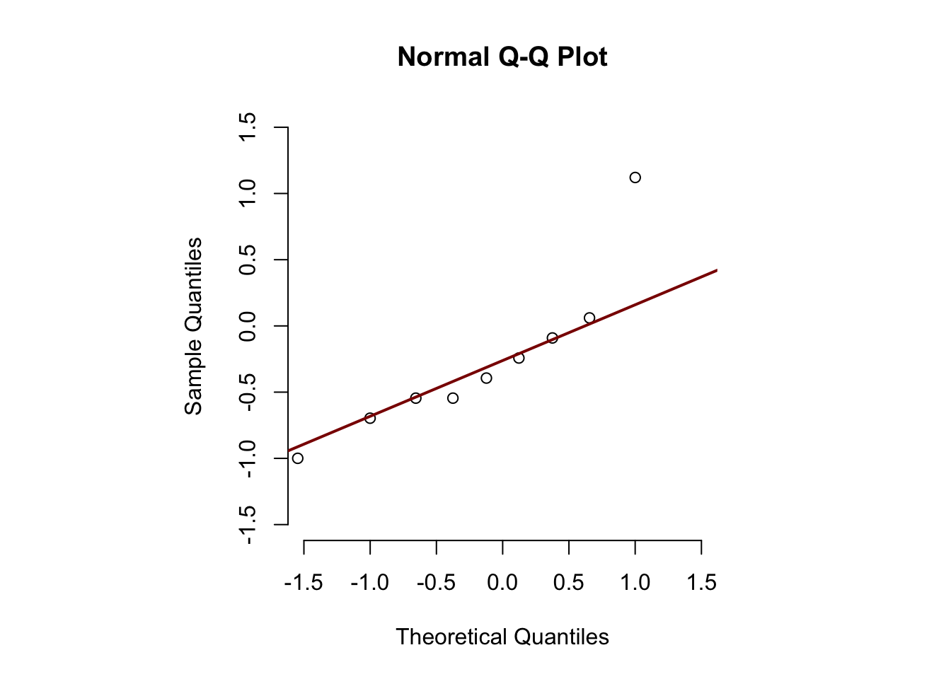
Normality

Shape of distribution (and no CLT)
Outliers
Illustration of consequences

Nonparametric tests

When assumptions are violated
- e.g., strong non-normality
When the variable is ordinal
- e.g., when playing Mario Kart
When unsure about outliers
- e.g., some observations with z \(\approx\) 3
Topic of my dissertation!

Parametric vs Nonparametric

Attribute	Parametric	Nonparametric
distribution	normally distributed	any distribution
sampling	random sample	random sample
sensitivity to outliers	yes	no
works with	large data sets	small and large data sets
speed	fast	slow

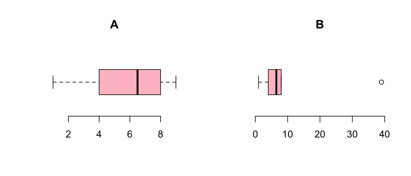
Ranking

A	1	4	6	7	8	9
B	1	4	6	7	8	39
-
rank(A)	1	2	3	4	5	6
rank(B)	1	2	3	4	5	6

Ties

index	1	2.0	3.0	4	5.0	6.0	7	8	9
x	11	42.0	42.0	62	73.0	73.0	84	84	84
ranks	1	2.5	2.5	4	5.5	5.5	8	8	8

\[\frac{2 + 3}{2} = 2.5, \frac{5 + 6}{2} = 5.5, \frac{7 + 8 + 9}{3} = 8\]

Procedure

Assumption: independent random samples.
Hypothesis:
\(H_0\) : equal population distributions (implies equal mean ranking)
\(H_A\) : unequal mean ranking (two sided)
\(H_A\) : higher mean ranking for one group.
Test statistic is difference between mean or sum of ranking.
Standardize test statistic to normal sampling distribution.
Calculate P-value one or two sided.
Conclude to reject \(H_0\) if \(p < \alpha\).

Wilcoxon rank-sum test

Independent 2 samples

Also known as the Mann-Whitney U test

Wilcoxon rank-sum test

Developed by Frank Wilcoxon the rank-sum test is an nonparametric alternative to the independent samples t-test.

By ranking all values and then summing the ranks per group, one would expect under the null hypothesis, that the sum of ranks is approximately equal.

After standardizing the test statistic (summed ranks for one group), we can use the standard normal distribution as the sampling distribution.

Example

Link

Test statistic W is the sum of ranks per group

rankSums <- aggregate(rankedBDI ~ Drug, data, sum)
rankSums

     Drug rankedBDI
1 Alcohol      90.5
2 Ecstasy     119.5

We can take the sum of ranks for the first group as W:

W <- rankSums[1, 2]
W

[1] 90.5

Subtracting the minimum score

JASP reports the value of U, which is W with its minimum value subtracted:

W.min <- sum(1:10); W.min

[1] 55

U <- W - W.min
U

[1] 35.5

Normal approximation for W

To calculate the Z-score we need to standardize the W. To do so we need the mean W and the standard error of W.

For this we need the sample sizes for each group.

n <- aggregate(rankedBDI ~ factor, data, length)

n.1 <- n$rankedBDI[1]
n.2 <- n$rankedBDI[2]

cbind(n.1, n.2)

     n.1 n.2
[1,]  10  10

Mean W under \(H_0\)

\[\bar{W}_s=\frac{n_1(n_1+n_2+1)}{2}\]

W.mean <- (n.1 * (n.1 + n.2 + 1)) / 2
W.mean # this is the middle point between the min and max value of W

[1] 105

W.max <- sum(11:20); W.max

[1] 155

W.min <- sum(1:10); W.min

[1] 55

SE W

\[{SE}_{\bar{W}_s}=\sqrt{ \frac{n_1 n_2 (n_1+n_2+1)}{12} }\]

W.se <- sqrt((n.1 * n.2 * (n.1 + n.2 + 1)) / 12)
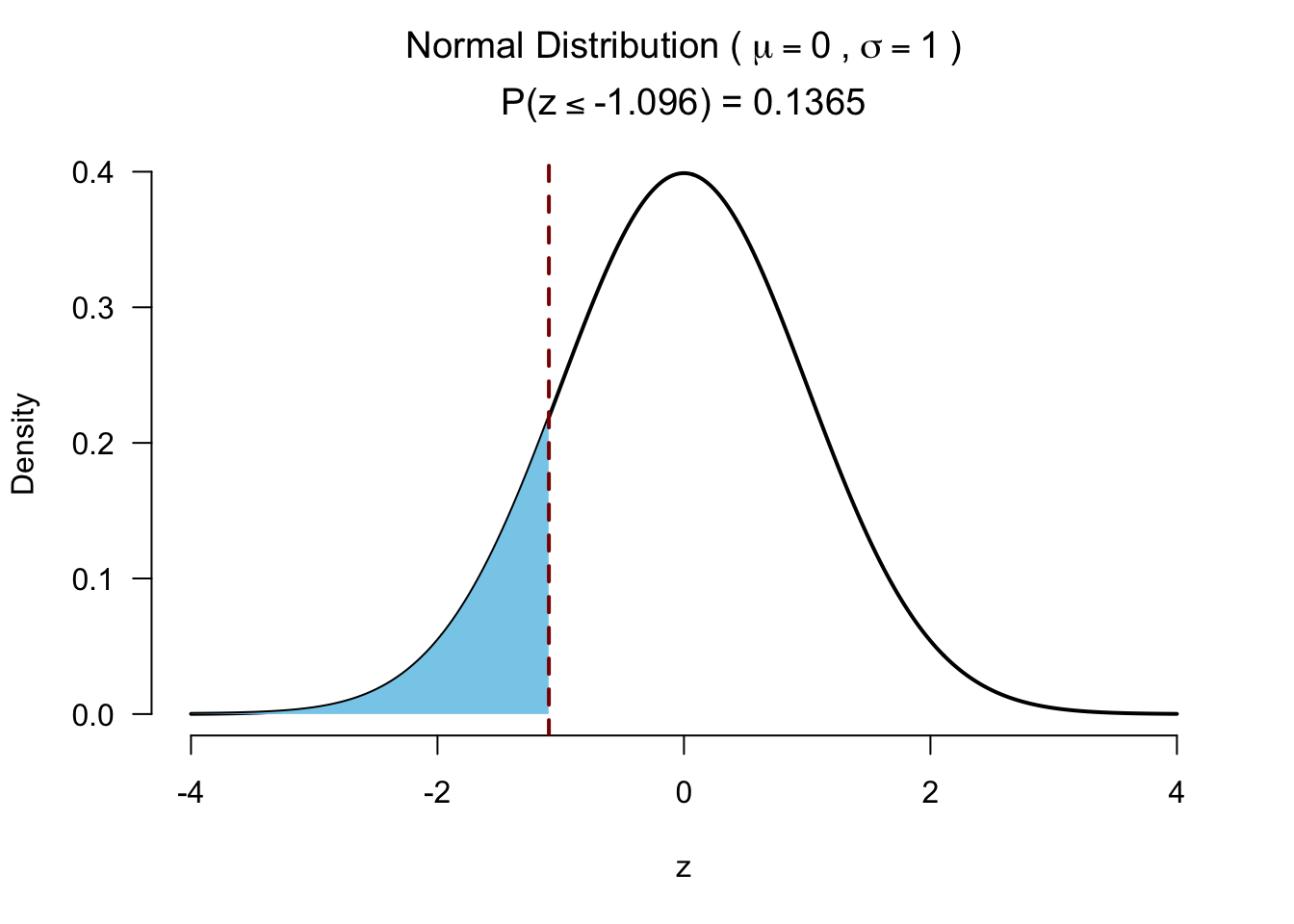
W.se

[1] 13.22876

Calculate Z

\[z = \frac{W - \bar{W}}{{SE}_W}\]

Which looks a lot like

\[\frac{X - \bar{X}}{{SE}_X} \text{or} \frac{b - \mu_{b}}{{SE}_b} \]

z <- (W - W.mean) / W.se
z

[1] -1.096097

Test for significance 2 sided

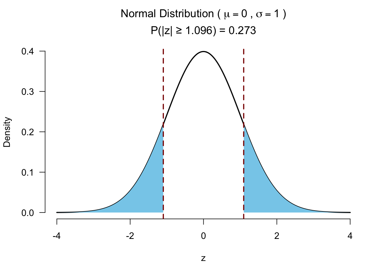
Test for significance 1 sided

Effect size rank-biserial correlation

\[r_{bs} = 1 - \frac{2*W}{n_1*n_2}\]

W <- W - W.min # use modern W
biserialCor <- 1 - (2*(W)) / (n.1*n.2);
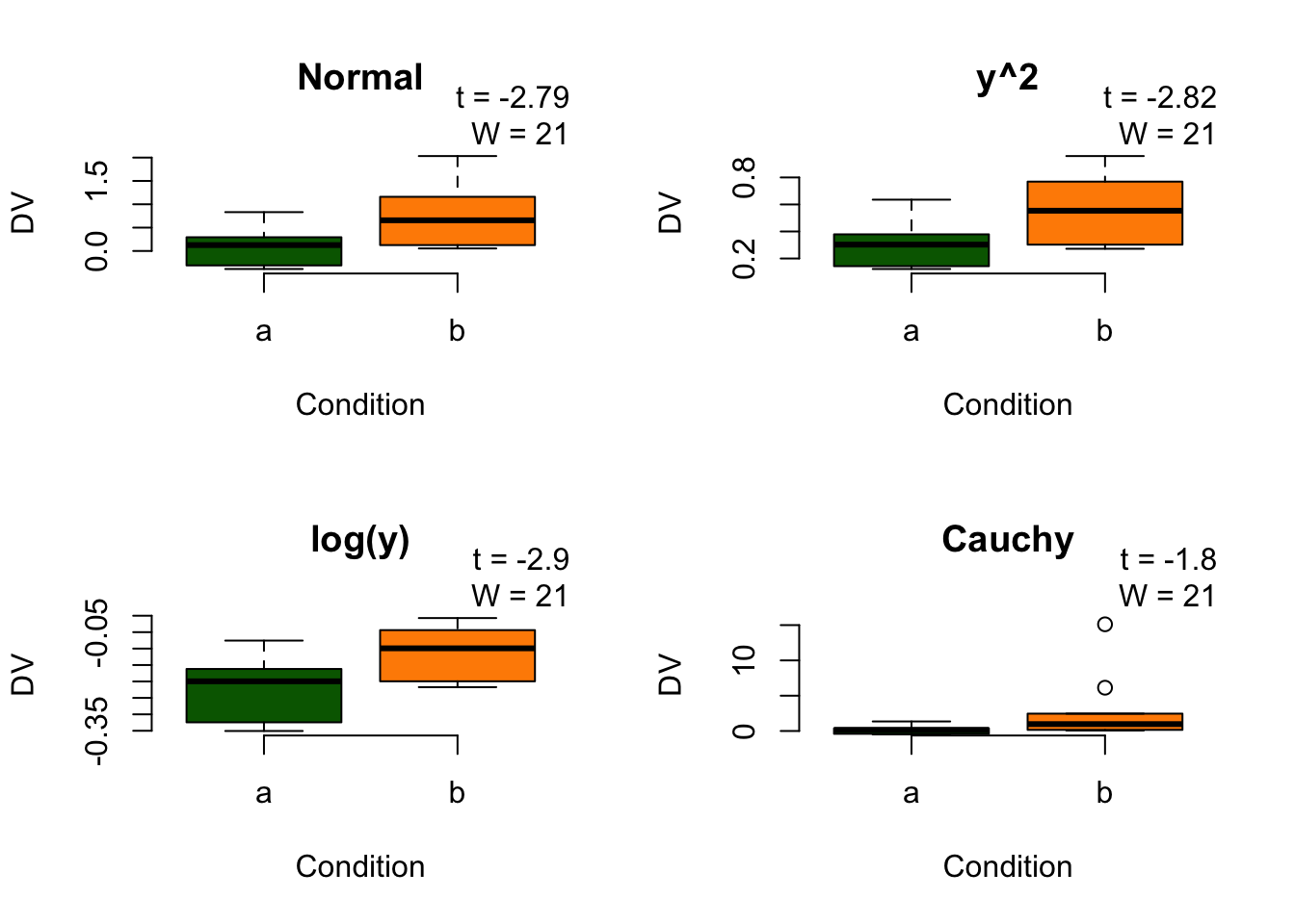
biserialCor

[1] 0.29

Robustness under monotonic transformations

Wilcoxon signed-rank test

Paired 2 samples

Wilcoxon signed-rank test

The Wilcoxon signed-rank test is a nonparametric alternative to the paired samples t-test. It assigns + or - signs to the difference between two repeated measures. By ranking the absolute differences and summing these ranks for the positive group, the null hypothesis is tested that both positive and negative differences are equal.

Example

The plot

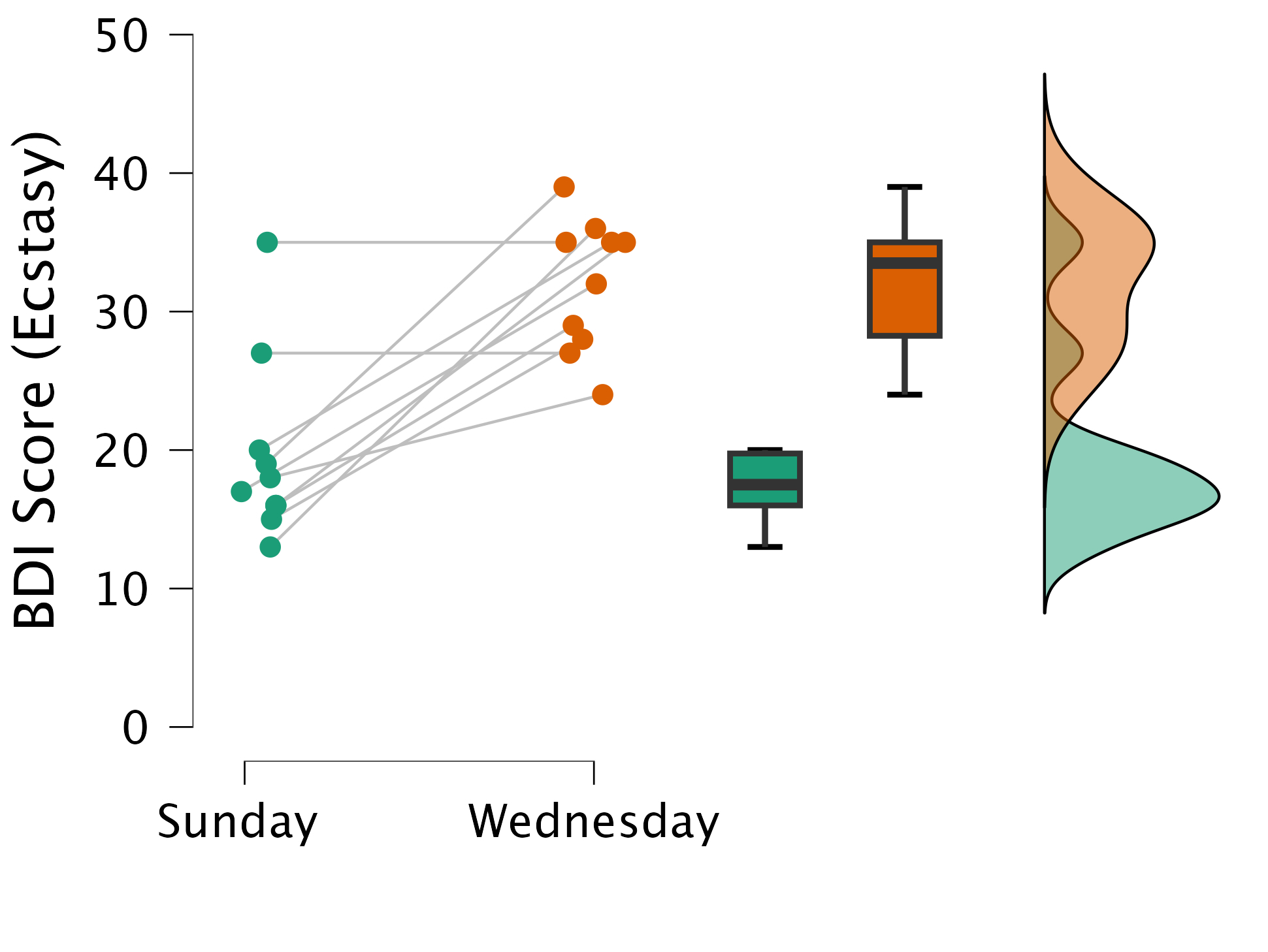
Calculate T

# Calculate difference in scores between first and second measure
data$diff = data$Sunday - data$Wednesday

# Calculate absolute difference in scores between first and second measure
data$abs.diff = abs(data$Sunday - data$Wednesday)

# Remove observations where the difference is 0
data <- data[data$diff != 0, ]

# Create rank variable
data$rank <- rank(data$abs.diff)

# Assign a '+' or a '-' to those values 
data$sign <- sign(data$Sunday - data$Wednesday)

The data

Link

Calculate \(T_+\)

# Calculate the sum of the positive ranks
T_pos <- sum(data$rank * (data$diff > 0))
T_pos

[1] 0

# Calculate N without 0 (no differences).
n <- nrow(data)
n

[1] 8

How likely is it to observe the lowest possible rank sum (0), for \(n=8\), if there is no difference in BDI between Sunday and Wednesday?

Calculate \(\bar{T}\) and \({SE}_{T}\)

\[\bar{T} = \frac{n(n+1)}{4}\]

T_mean <- (n*(n+1))/4
T_mean

[1] 18

T_mean is the middle point between the minimum (0) and maximum possible (36) value for T

\[{SE}_{T} = \sqrt{\frac{n(n+1)(2n+1)}{24}}\]

SE_T <- sqrt( (n*(n+1)*(2*n+1)) / 24)

Calculate Z

\[z = \frac{T_+ - \bar{T}}{{SE}_T}\]

z <- (T_pos - T_mean)/SE_T
z

[1] -2.520504

Test for significance

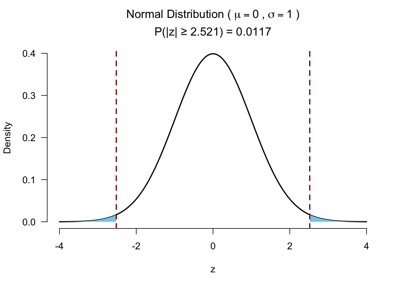
Effect size

Matched rank-biserial correlation

\[r = \frac{T_+ - T_- }{T_+ + T_-}\]

Here \(T_+\) is the sum of the positive ranks (i.e., where Sunday > Wednesday), which do not exist. \(T_-\) is the sum of the negative ranks, which is 36. We have a maximum negative correlation (i.e., everybody scored lower on Wednesday).

T_neg <- sum(data$rank * (data$diff < 0)) # sum negative ranks
T_neg

[1] 36

rbis <- (T_pos - T_neg) / (T_pos + T_neg)
rbis

[1] -1

Kruskal–Wallis test

Independent >2 samples

Kruskal–Wallis test

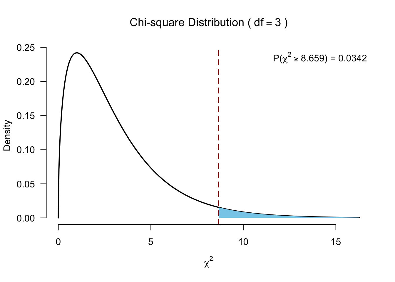
Created by William Henry Kruskal (L) and Wilson Allen Wallis (R), the Kruskal-Wallis test is a nonparametric alternative to the independent one-way ANOVA.

The Kruskal-Wallis test essentially subtracts the expected mean ranking from each oberved mean ranking, which is \(\chi^2\) distributed.

Assign ranks

# Assign ranks
data$ranks <- rank(data$Testosterone)

The data

Link

Calculate H

\[H = \frac{12}{N(N+1)} \sum_{i=1}^k \frac{R_i^2}{n_i} - 3(N+1)\]

\(N\) total sample size
\(n_i\) sample size per group
\(k\) number of groups
\(R_i\) rank sums per group

Calculate H

# Now we need the sum of the ranks per group.
R.i <- aggregate(ranks ~ Soya, data = data, sum)$ranks
R.i

[1] 883 883 547 927

# De total sample size N is:
N <- nrow(data)

# And the sample size per group is n_i:
n.i <- aggregate(Testosterone ~ Soya, data=data, length)$Testosterone
n.i

[1] 20 20 20 20

Calculate H

\[H = \frac{12}{N(N+1)} \sum_{i=1}^k \frac{R_i^2}{n_i} - 3(N+1)\]

H <- ( 12/(N*(N+1)) ) * sum(R.i^2/n.i) - 3*(N+1)
H

[1] 8.658889

And the degrees of freedom

k  <- 4
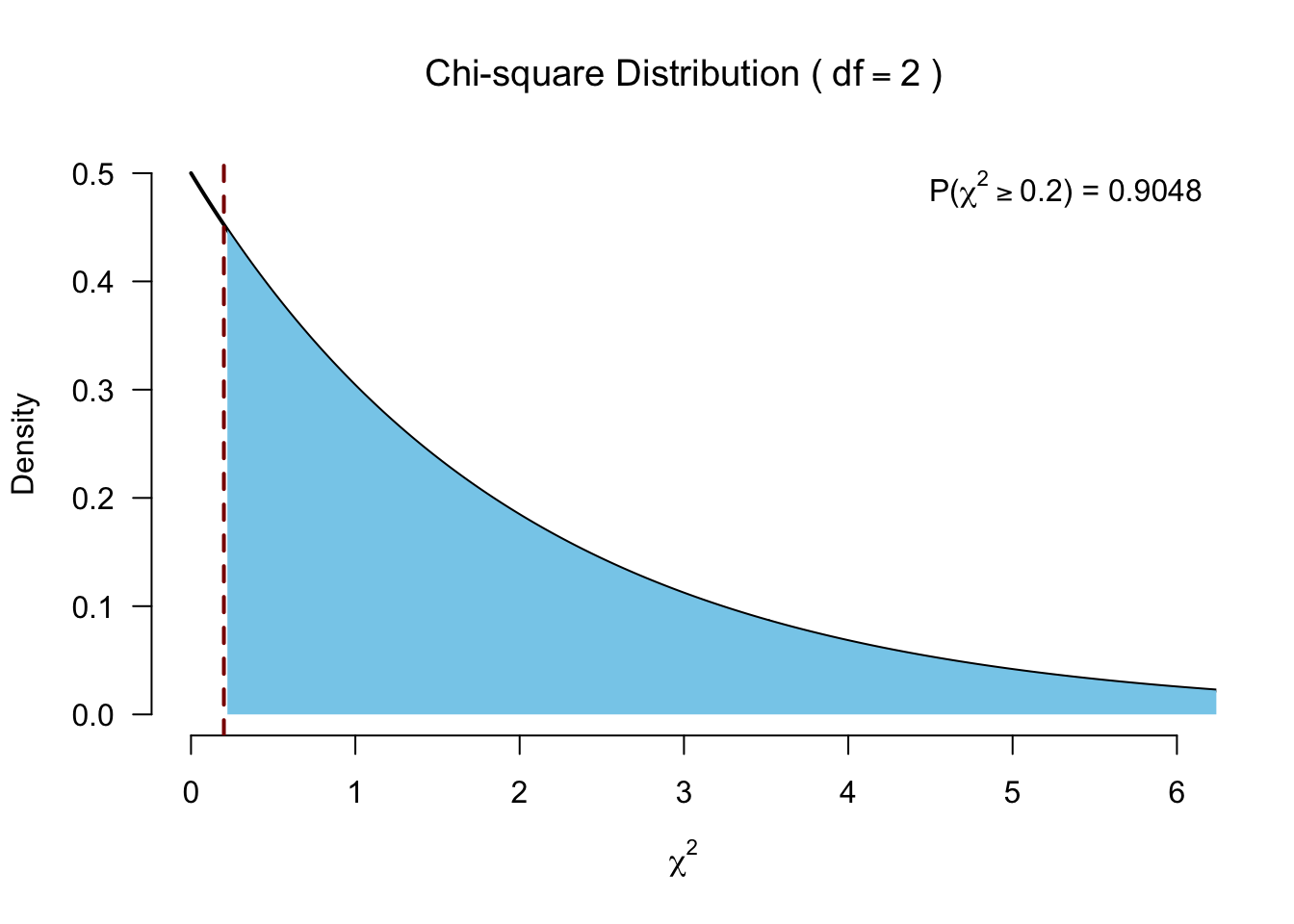
df <- k - 1

Test for significance

Follow-up?

Dunn’s post hoc test:
- Pairwise Mann-Whitney tests with adjusted p-values

Friedman’s ANOVA

Paired >2 samples

Friedman’s ANOVA

Created by William Frederick Friedman the Friedman’s ANOVA is a nonparametric alternative to the repeated one-way ANOVA.

Just like the Kruskal-Wallis test, Friedman’s ANOVA, subtracts the expected mean ranking from the calculated observed mean ranking, which is also \(\chi^2\) distributed.

The data

Link

Assign ranks

Rank within each participant (i.e., within each row).

# Rank for each person
ranks <- t(apply(data, 1, rank))

The data with ranks

Calculate \(F_r\)

\[F_r = \left[ \frac{12}{Nk(k+1)} \sum_{i=1}^k R_i^2 \right] - 3N(k+1)\]

\(N\) total number of subjects
\(k\) number of groups
\(R_i\) rank sums for each group

–> We sum the ranks for each of the three experimental conditions (and apply some standardizations).

Calculate \(F_r\)

Calculate ranks sum per condition and \(N\).

R.i <- apply(ranks, 2, sum)
R.i

T0_R T1_R T2_R 
  19   20   21

# N is number of participants
N <- 10

Calculate \(F_r\) (without adjusting for ties)

\[F_r = \left[ \frac{12}{Nk(k+1)} \sum_{i=1}^k R_i^2 \right] - 3N(k+1)\]

k <- 3
F.r <- ( ( 12/(N*k*(k+1)) ) * sum(R.i^2) ) - ( 3*N*(k+1) )
F.r

[1] 0.2

Adjusting for ties (just for fun)

\[ \frac{(k-1) \sum_i^k (R_i - \frac{b(k+1))}{2})^2}{\sum_i^b \sum_j^k (R_{ij}^2) - \frac{bk(k+1)^2}{4}} \]

k <- 3
b <- 10
F.r <- (sum ((R.i - ((b*(k+1))/2) )^2) * (k-1)) / (sum((ranks^2)) - (b*k *(k+1)^2) / 4)
F.r

[1] 0.2

And the degrees of freedom

df <- k - 1

Test for significance

Post hoc tests?

Conover test
Follow up with Wilcoxon signed-rank tests!

Closing

Recap

Non-parametric tests are rank-based, which means they are robust to:
- Non-normality
- Transformations of the data
- Outliers

Recommended Exercises

Exercise 15.1, Exercise 15.2, Exercise 15.4, Exercise 15.11

Contact