22. Multiple regression
Block 3: Life is Continuous
- Regression with multiple predictors
- Interaction effects
- Mediation effects
- Chi-square
- Bayes!
In this lecture we aim to:
- Repeat some regression
- Look at multiple predictors
- Show these in JASP
Reading: Chapter 8
Multiple regression
\(\LARGE{\text{outcome} = \text{model prediction} + \text{error}}\)
In statistics, linear regression is a linear approach for modeling the relationship between a scalar dependent variable y and one or more explanatory variables denoted X.
\(\LARGE{Y_i = \beta_0 + \beta_1 X_{1i} + \beta_2 X_{2i} + \dotso + \beta_n X_{ni} + \epsilon_i}\)
In linear regression, the relationships are modeled using linear predictor functions whose unknown model parameters \(\beta\)’s are estimated from the data.
Source: wikipedia
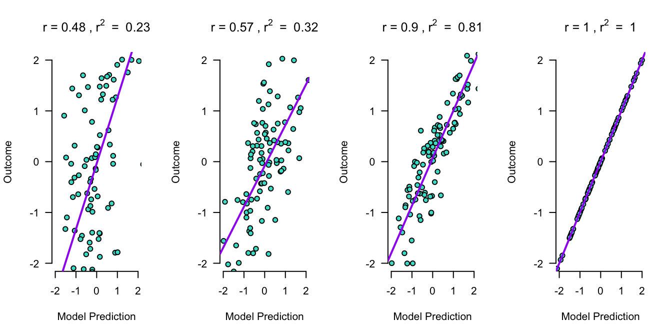
Outcome vs Model Prediction
Assumptions
A selection from Field (8.3 Bias in linear models):
For simple regression
- Sensitivity
- Homoscedasticity
- See here for further illustration
- Linearity
- Normality
Additionally, for multiple regression
- Multicollinearity (Section 8.9)
Multicollinearity
To adhere to the multicollinearity assumption, there must not be a too high linear relation between the predictor variables.
This can be assessed through:
- Correlations
- Matrix scatterplot
- Collinearity diagnostics
- VIF: max < 10, mean < 1
- Tolerance > 0.2 -> good
- Tolerance = \(\frac{1}{VIF}\)

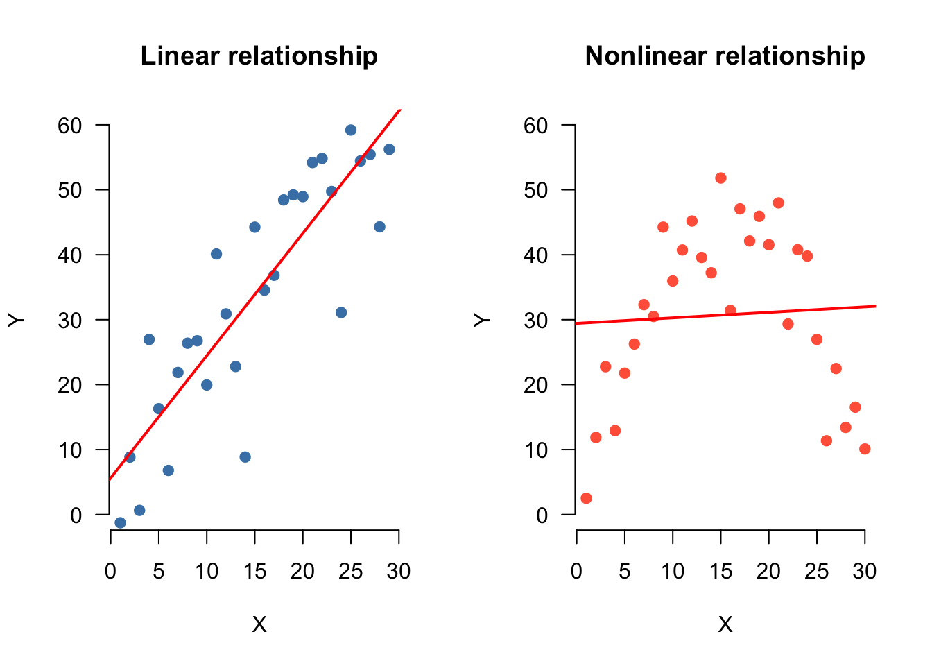
Linearity
For the linearity assumption to hold, the predictors must have a linear relation to the outcome variable.
This can be checked through:
- Correlations
- Matrix scatterplot with predictors and outcome variable
Example
Predict album sales (1,000 copies) based on airplay (no. plays) and adverts ($1,000).
Read data
Regression model
Predict album sales based on airplay and adverts.
\[{sales}_i = b_0 + b_1 {airplay}_i + b_2 {adverts}_i + \epsilon_i\]
fit <- lm(sales ~ airplay + adverts, data = data)What is the model?
The beta coefficients are:
- \(b_0\) (intercept) = 41.12
- \(b_1\) = 3.59
- \(b_2\) = 0.09.
How to visualize??
- When we plot 1 predictors + DV, we plot in 2 dimensions, and we summarize the relationship by a line
- When we plot 2 predictors + DV, we plot in 3 dimensions, and we summarize the relationship by a plane
- … ???
Visual
What are the predicted values based on this model
\(\widehat{\text{album sales}} = b_0 + b_1 \text{airplay} + b_2 \text{adverts}\)
predicted.sales <- b.0 + b.1 * airplay + b.2 * adverts\(\text{model prediction} = \widehat{\text{album sales}}\)
Apply regression model
\(\widehat{\text{album sales}} = b_0 + b_1 \text{airplay} + b_2 \text{adverts}\)
\(\widehat{\text{album sales}} = 41.12 + 3.59 \times \text{airplay} + 0.09 \times \text{adverts} = 196.413\)
How far are we off?
error <- sales - predicted.salesOutcome = Model Prediction + Error
Is that true?
sales == predicted.sales + error [1] TRUE TRUE TRUE TRUE TRUE TRUE TRUE TRUE TRUE TRUE TRUE TRUE TRUE TRUE TRUE
[16] TRUE TRUE TRUE TRUE TRUE TRUE TRUE TRUE TRUE TRUE TRUE TRUE TRUE TRUE TRUE
[31] TRUE TRUE TRUE TRUE TRUE TRUE TRUE TRUE TRUE TRUE TRUE TRUE TRUE TRUE TRUE
[46] TRUE TRUE TRUE TRUE TRUE TRUE TRUE TRUE TRUE TRUE TRUE TRUE TRUE TRUE TRUE
[61] TRUE TRUE TRUE TRUE TRUE TRUE TRUE TRUE TRUE TRUE TRUE TRUE TRUE TRUE TRUE
[76] TRUE TRUE TRUE TRUE TRUE TRUE TRUE TRUE TRUE TRUE TRUE TRUE TRUE TRUE TRUE
[91] TRUE TRUE TRUE TRUE TRUE TRUE TRUE TRUE TRUE TRUE TRUE TRUE TRUE TRUE TRUE
[106] TRUE TRUE TRUE TRUE TRUE TRUE TRUE TRUE TRUE TRUE TRUE TRUE TRUE TRUE TRUE
[121] TRUE TRUE TRUE TRUE TRUE TRUE TRUE TRUE TRUE TRUE TRUE TRUE TRUE TRUE TRUE
[136] TRUE TRUE TRUE TRUE TRUE TRUE TRUE TRUE TRUE TRUE TRUE TRUE TRUE TRUE TRUE
[151] TRUE TRUE TRUE TRUE TRUE TRUE TRUE TRUE TRUE TRUE TRUE TRUE TRUE TRUE TRUE
[166] TRUE TRUE TRUE TRUE TRUE TRUE TRUE TRUE TRUE TRUE TRUE TRUE TRUE TRUE TRUE
[181] TRUE TRUE TRUE TRUE TRUE TRUE TRUE TRUE TRUE TRUE TRUE TRUE TRUE TRUE TRUE
[196] TRUE TRUE TRUE TRUE TRUE
- Yes!
Visual (subset of 10 albums)
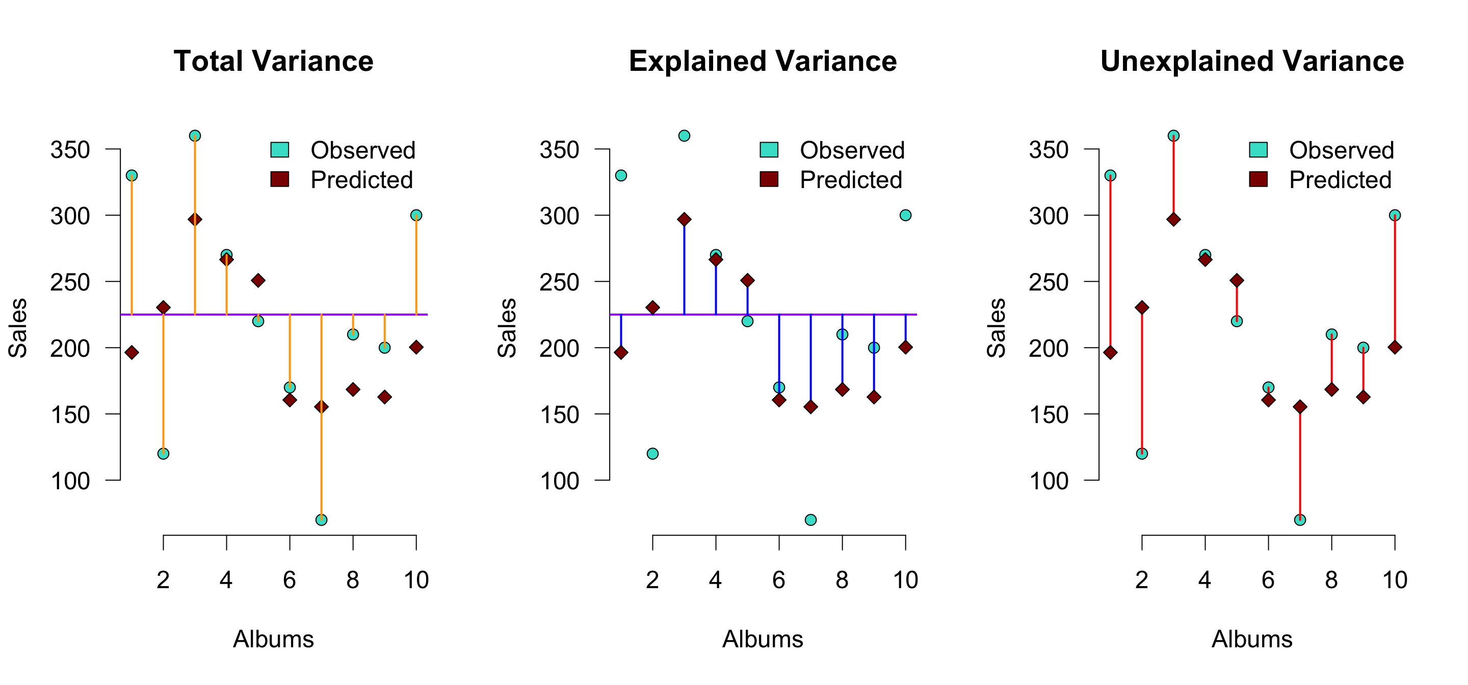
\(r^2\) is the proportion of blue to orange, while \(1 - r^2\) is the proportion of red to orange
Explained variance
The explained variance is the deviation of the estimated model outcome compared to the grand mean.
To get a percentage of explained variance, it must be compared to the total variance. In terms of squares:
\(\frac{{SS}_{model}}{{SS}_{total}}\)
We also call this: \(r^2\) or \(R^2\).
Why?
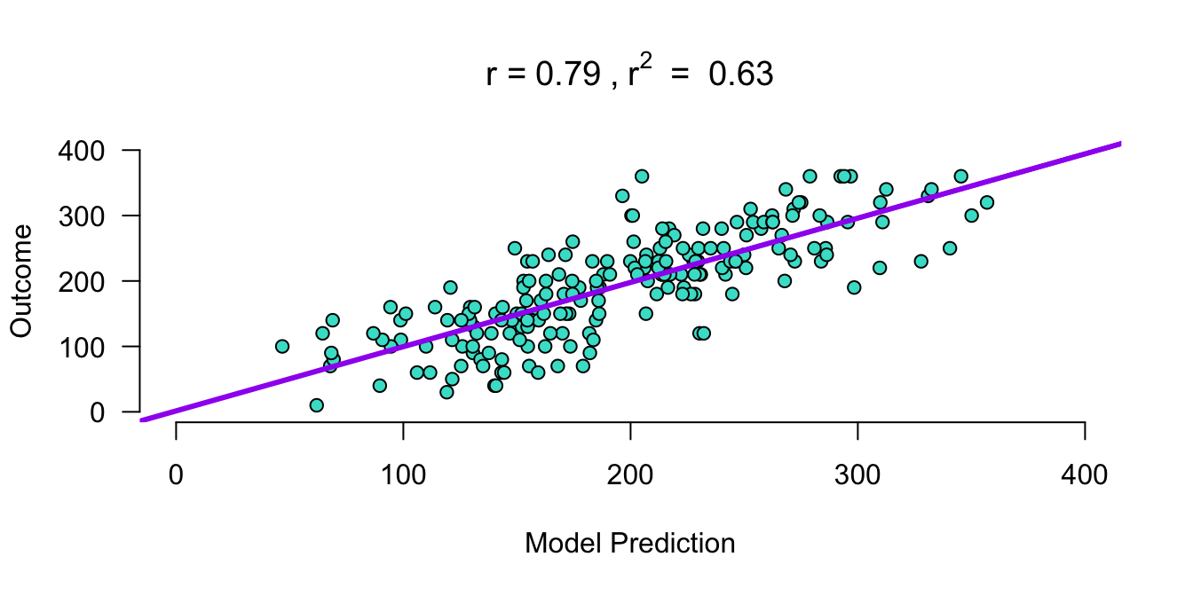
r <- cor(sales, predicted.sales)
r^2
[1] 0.62913Explained variance
JASP
![]()
Closing
Recap
- In linear regression, we can build multiple models and look at their fit
- Just as in ANOVA, when we have multiple predictors we look out for:
- Dependence between predictors
- Interaction effects
Recommended Exercises
Contact
