26. Moderation
2025-11-07
Model
\(\definecolor{red}{RGB}{255,0,0} \definecolor{black}{RGB}{0,0,0} \color{black}Out_i = b_0 + b_1 Pred_i + b_2 Mod_i + \color{red}b_3 Pred_i \times Mod_i \color{black}+ \epsilon_i\)
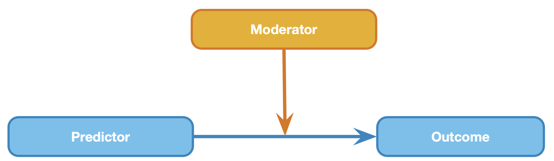
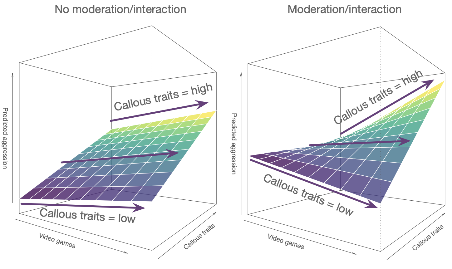
Model
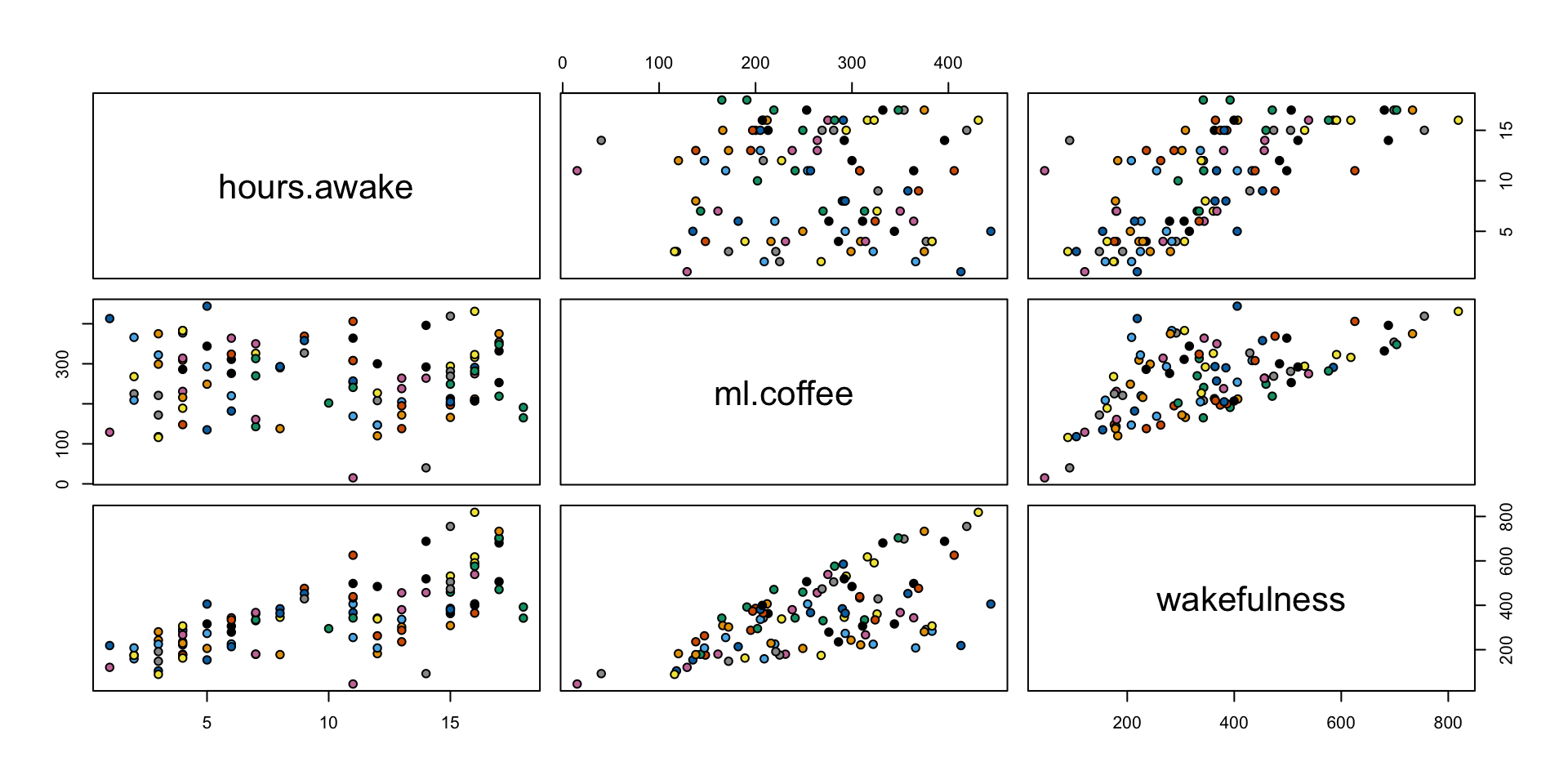
Scatterplots
Expected values
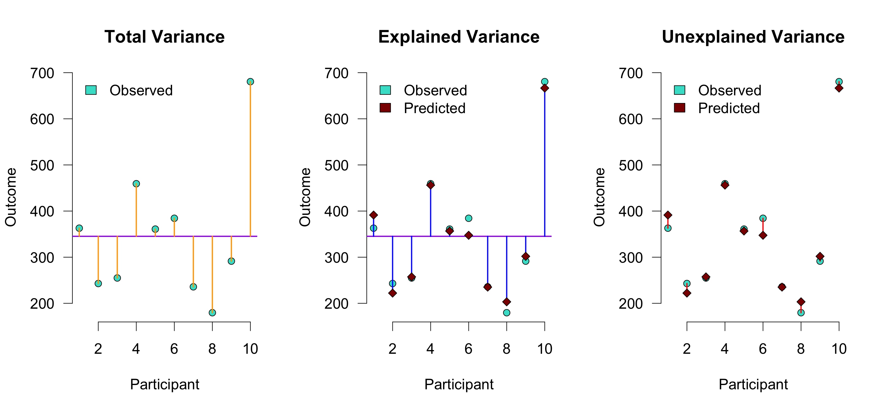
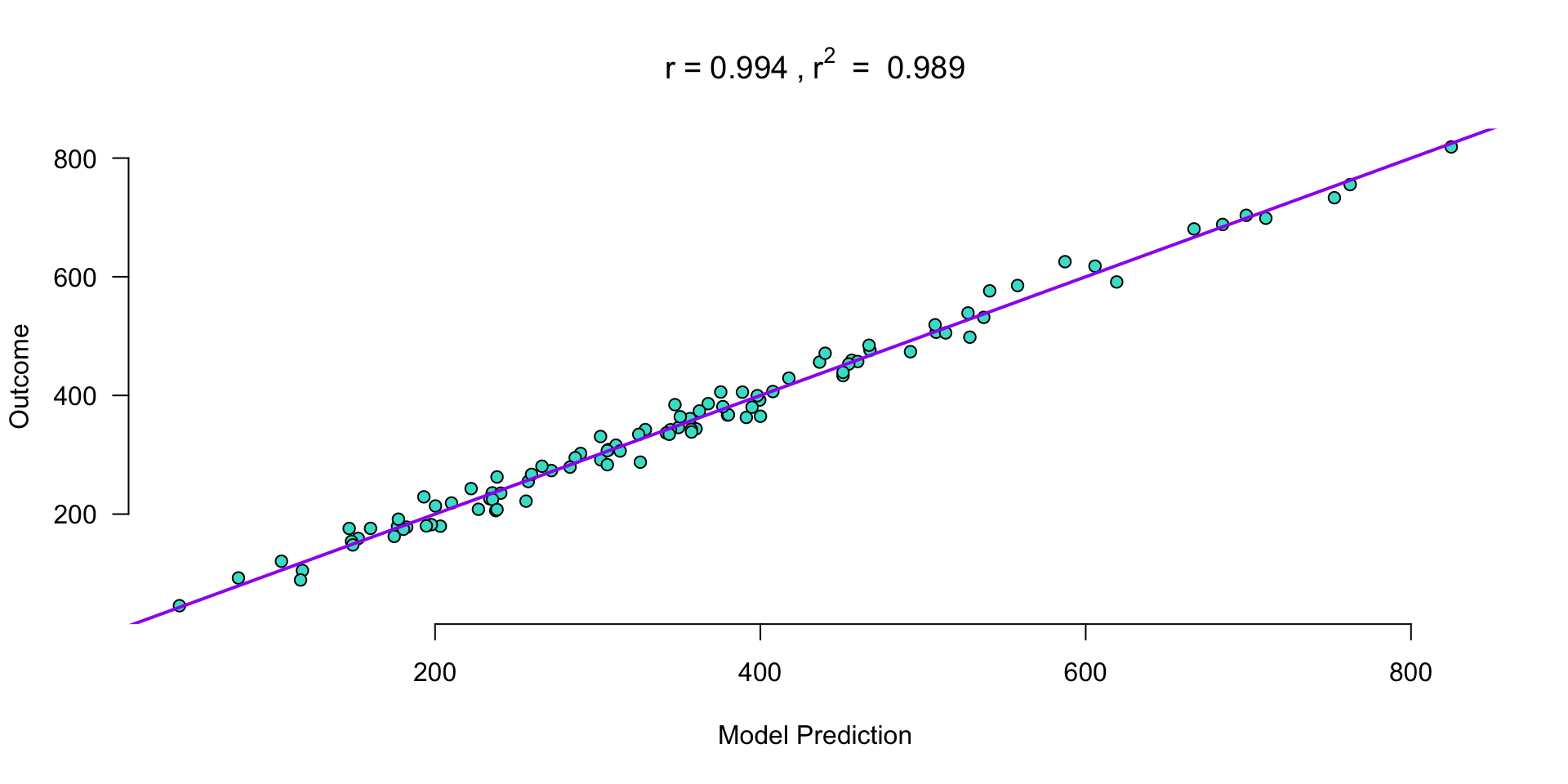
\(r^2\) is the proportion of blue to orange, while \(1 - r^2\) is the proportion of red to orange
Expected vs. observed
Demonstration
- Moderation in Process module
- Moderation in regression module
- Equivalences in regression
![]()
Contact

![]()