28. Chi-squared test
Contingency Tables
In this lecture we aim to:
- Discuss association between categorical variables
- Contingency tables
- Show this test in JASP
Reading: Chapter 16
\(\chi^2\) test
Relation between categorical variables
\(\chi^2\) test
A “chi-squared test”, also written as \(\chi^2\) test, is any statistical hypothesis test wherein the sampling distribution of the test statistic is a chi-squared distribution when the null hypothesis is true. Without other qualification, ‘chi-squared test’ often is used as short for Pearson’s chi-squared test.
Chi-squared tests are often constructed from a Lack-of-fit sum of squared errors. A chi-squared test can be used to attempt rejection of the null hypothesis that the data are independent.
Source: wikipedia
\(\chi^2\) test statistic
\(\chi^2 = \sum \frac{(\text{observed}_{ij} - \text{model}_{ij})^2}{\text{model}_{ij}}\)
Contingency table
\(\text{observed}_{ij} = \begin{pmatrix} o_{11} & o_{12} & \cdots & o_{1j} \\ o_{21} & o_{22} & \cdots & o_{2j} \\ \vdots & \vdots & \ddots & \vdots \\ o_{i1} & o_{i2} & \cdots & o_{ij} \end{pmatrix}\)
\(\text{model}_{ij} = \begin{pmatrix} m_{11} & m_{12} & \cdots & m_{1j} \\ m_{21} & m_{22} & \cdots & m_{2j} \\ \vdots & \vdots & \ddots & \vdots \\ m_{i1} & m_{i2} & \cdots & m_{ij} \end{pmatrix}\)
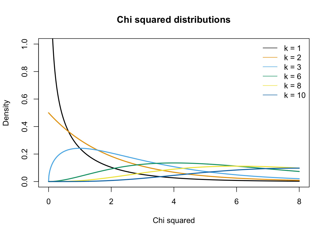
\(\chi^2\) distribution
The \(\chi^2\) distribution describes the test statistic under the assumption of \(H_0\), given the degrees of freedom.
\(df = (r - 1) (c - 1)\) where \(r\) is the number of rows and \(c\) the number of columns.
Experiment

Data
Calculating \(\chi^2\)
observed <- table(results[, c("Lecture", "Personality")])
observed
Personality
Lecture Extrovert Introvert
Digital 10 13
Live 13 16\(\text{observed}_{ij} = \begin{pmatrix} 10 & 13 \\ 13 & 16 \\ \end{pmatrix}\)
Calculating the model
\(\text{model}_{ij} = E_{ij} = \frac{\text{row total}_i \times \text{column total}_j}{n }\)
n <- sum(observed)
totExt <- colSums(observed)[1]
totInt <- colSums(observed)[2]
totDig <- rowSums(observed)[1]
totLiv <- rowSums(observed)[2]
addmargins(observed) Personality
Lecture Extrovert Introvert Sum
Digital 10 13 23
Live 13 16 29
Sum 23 29 52Calculating the model
\(\text{model}_{ij} = E_{ij} = \frac{\text{row total}_i \times \text{column total}_j}{n }\)
modelPredictions <- matrix( c((totExt * totDig) / n,
(totExt * totLiv) / n,
(totInt * totDig) / n,
(totInt * totLiv) / n), 2, 2,
byrow=FALSE, dimnames = dimnames(observed)
)
modelPredictions Personality
Lecture Extrovert Introvert
Digital 10.17308 12.82692
Live 12.82692 16.17308\(\text{model}_{ij} = \begin{pmatrix} 10.1730769 & 12.8269231 \\ 12.8269231 & 16.1730769 \\ \end{pmatrix}\)
Error = Observed - Model
observed Personality
Lecture Extrovert Introvert
Digital 10 13
Live 13 16modelPredictions Personality
Lecture Extrovert Introvert
Digital 10.17308 12.82692
Live 12.82692 16.17308observed - modelPredictions Personality
Lecture Extrovert Introvert
Digital -0.1730769 0.1730769
Live 0.1730769 -0.1730769Calculating \(\chi^2\)
\(\chi^2 = \sum \frac{(\text{observed}_{ij} - \text{model}_{ij})^2}{\text{model}_{ij}}\)
# Calculate chi squared
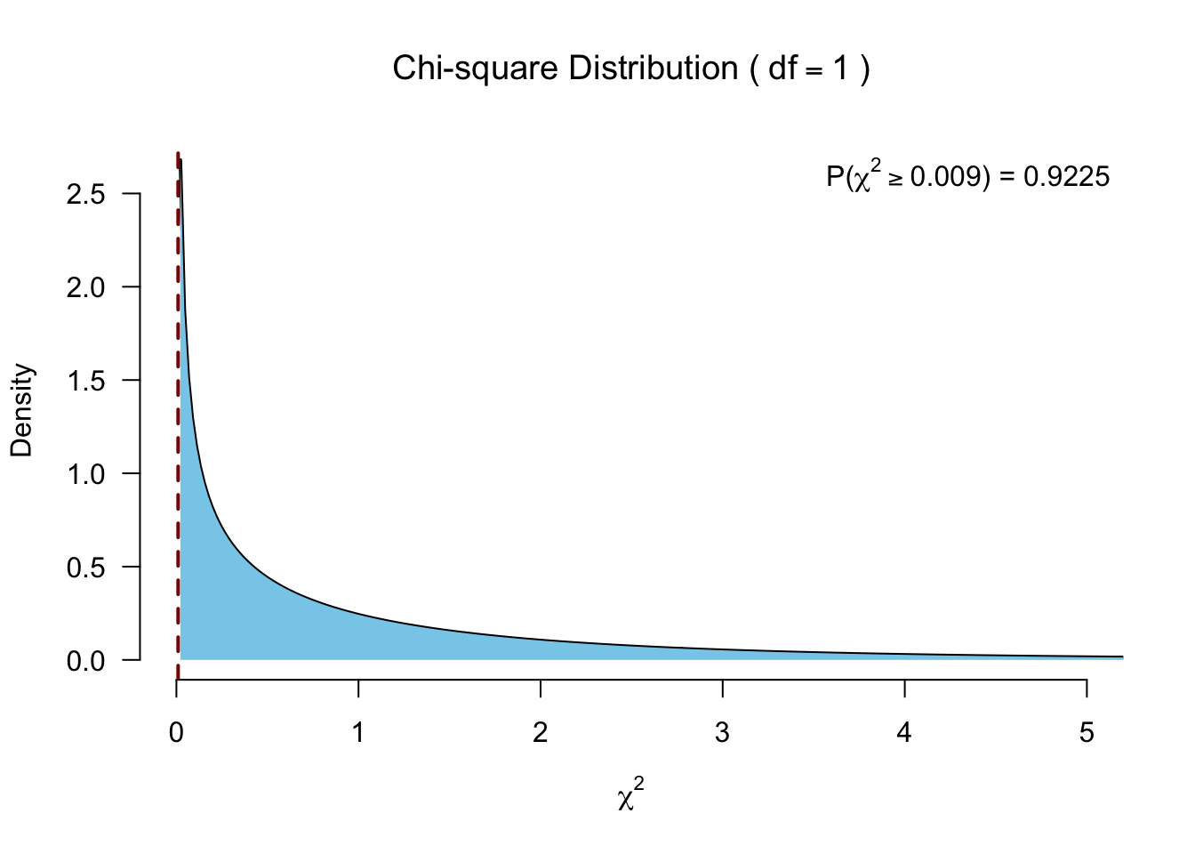
chi.squared <- sum((observed - modelPredictions)^2 / modelPredictions)
chi.squared[1] 0.00946753Testing for significance
\(df = (r - 1) (c - 1)\)
\(P\)-value
Fisher’s exact test
Calculates exact \(\chi^2\) for small samples (at least one cell of the table has an expected count smaller than 5), when the \(\chi^2\) approximation does not yet suffice.
Calculate all possible permutations.
- Exptected cell size < 5
Yates’s correction
For 2 x 2 contingency tables, Yates’s correction is to prevent overestimation of statistical significance for small data. Unfortunately, Yates’s correction may tend to overcorrect (i.e., produce an overly conservative result), and is not really recommended anymore (see Section 16.3.5).
\(\chi^2 = \sum \frac{ ( | \text{observed}_{ij} - \text{model}_{ij} | - .5)^2}{\text{model}_{ij}}\)
[1] 0.03377921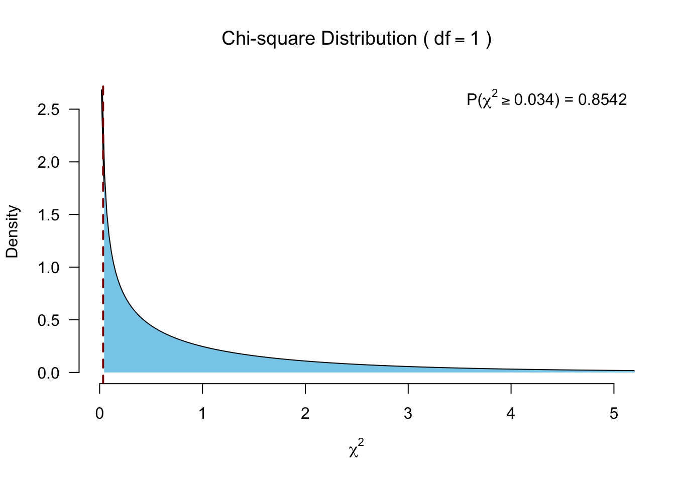
Standardized residuals
\(\text{standardized residuals} = \frac{ \text{observed}_{ij} - \text{model}_{ij} }{ \sqrt{ \text{model}_{ij} } }\)
(observed - modelPredictions) / sqrt(modelPredictions) Personality
Lecture Extrovert Introvert
Digital -0.05426415 0.04832567
Live 0.04832567 -0.04303708Effect size
Odds ratio based on the observed values
odds <- round( observed, 2); odds Personality
Lecture Extrovert Introvert
Digital 10 13
Live 13 16\(\begin{pmatrix} a & b \\ c & d \\ \end{pmatrix}\)
\(OR = \frac{a \times d}{b \times c} = \frac{10 \times 16}{13 \times 13} = 0.9467456\)
Odds
         Personality
Lecture   Extrovert Introvert
  Digital        10        13
Live 13 16The extrovert/introvert ratio for digital and live audiences:
- Digital \(\text{Odds}_{EI} = \frac{ 10 }{ 13 }\) = 0.7692308
- Live \(\text{Odds}_{EI} = \frac{ 13 }{ 16 }\) = 0.8125
In the digital responses, there are +- 0.77 times as many extroverts than introverts. In the live responses, there are +- 0.81 times as many extroverts than introverts.
Odds
         Personality
Lecture   Extrovert Introvert
  Digital        10        13
Live 13 16Alternatively, we can look at the ratio’s of digital/live for extroverts and introverts:
- Extrovert \(\text{Odds}_{DL} = \frac{ 10 }{ 13 }\) = 0.7692308
- Introvert \(\text{Odds}_{DL} = \frac{ 13 }{ 16 }\) = 0.8125
For the extroverts, there are +- 0.77 times as many digital viewers than live viewers. For the introverts, there are +- 0.81 times as many digital viewers than live viewers.
Odds ratio
Is the ratio of these odds.
\(OR = \frac{\text{digital}}{\text{live}} = \frac{0.7692308}{0.8125} = \frac{\text{extrovert}}{\text{introvert}} = \frac{0.7692308}{0.8125} = 0.9467456\)
For these data, extroverts were approximately 0.95 times more likely to watch digitally, compared to introverts. The odds ratio also accounts for the scores in both conditions—watching digitally and watching live—by comparing the odds of watching digitally to live viewing across both personality types.
Closing
Recap
- Chi-square test assesses categorical associations
- Can be used to assess (in)dependence between predictors
- Has test statistic (\(\chi^2\)) + effect size (odds ratio)
Recommended Exercises
Contact
