mu     <- 120
n      <- length(IQ.next.to.you)
x      <- IQ.next.to.you
mean_x <- mean(x, na.rm = TRUE)
sd_x   <- sd(x, na.rm = TRUE)
cbind(n, mean_x, sd_x)
n mean_x sd_x
[1,] 86 113.2209 27.91685University of Amsterdam
29 September 2026
In this lecture we aim to:
Reading: Chapter 9 (§9.1–9.14)
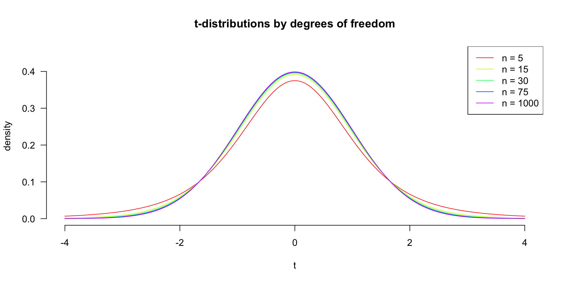
Fatter tails for small \(n\) (few degrees of freedom); converges to the standard normal as \(n\) grows.
Compare 1 group mean to a hypothesized value

\[\text{outcome} = \text{model} + \text{error}\]
What does each model predict?
\(H_0: \text{model} = 120\)
Uses a postulated value
\(H_A: \text{model} = \bar{x}\)
Uses the observed data
Can you phrase research questions that would lead you to each of these three versions of \(H_A\)?
We use the one-sample t-test to compare the sample mean \(\bar{x}\) to the mean that is hypothesized by \(H_0\): \(\mu = 120\). Let’s take a look at our sample:
mu <- 120
n <- length(IQ.next.to.you)
x <- IQ.next.to.you
mean_x <- mean(x, na.rm = TRUE)
sd_x <- sd(x, na.rm = TRUE)
cbind(n, mean_x, sd_x) n mean_x sd_x
[1,] 86 113.2209 27.91685Does this mean differ significantly from \(H_0:\) \(\mu = 120\)?
\[T_{n-1} = \frac{\bar{x}-\mu}{SE_x} = \frac{\bar{x}-\mu}{s_x / \sqrt{n}} = \frac{113.22 - 120 }{27.92 / \sqrt{86}}\]
So the t-statistic represents the deviation of the sample mean \(\bar{x}\) from the population mean \(\mu\), considering the sample size.
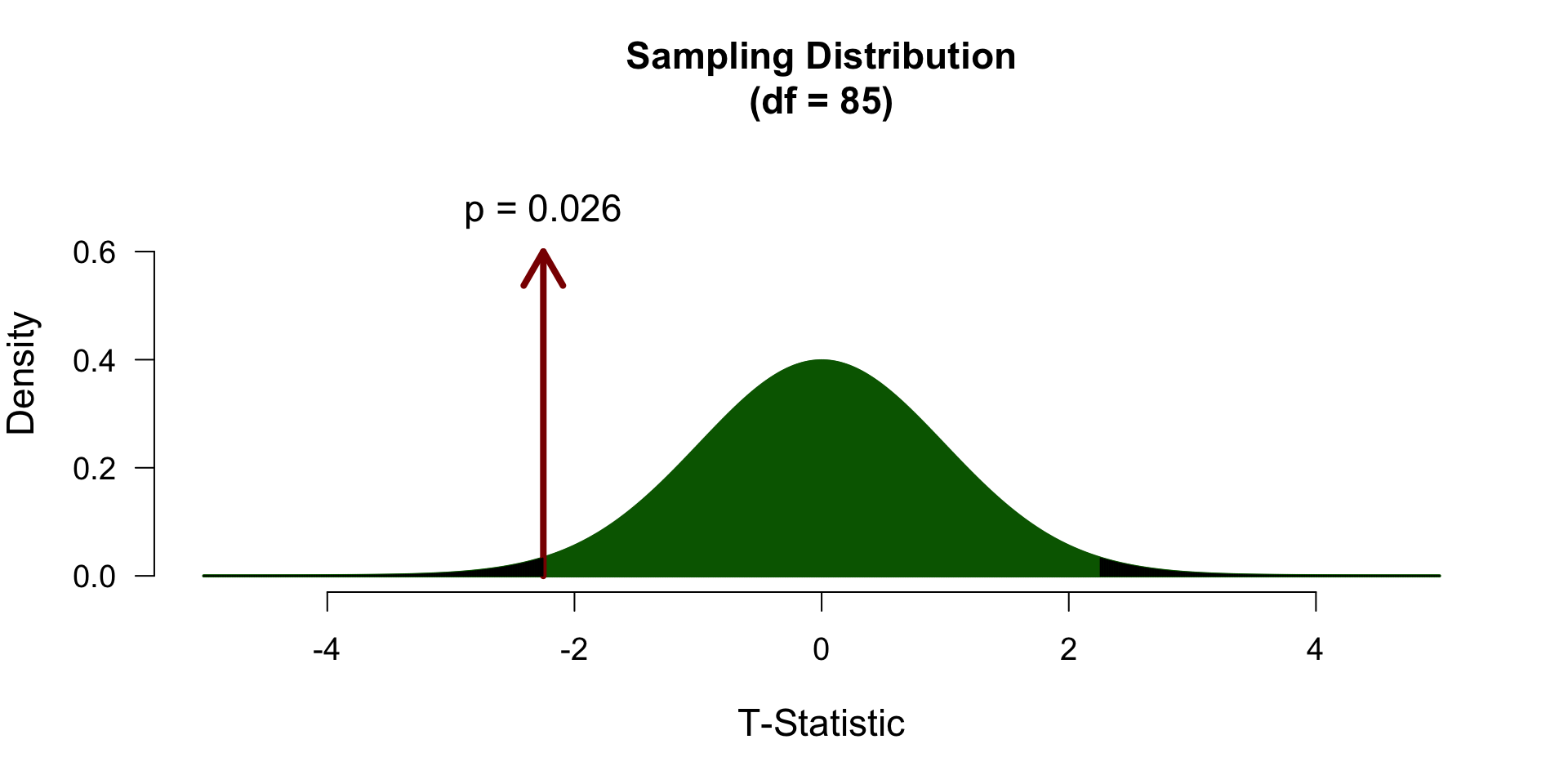
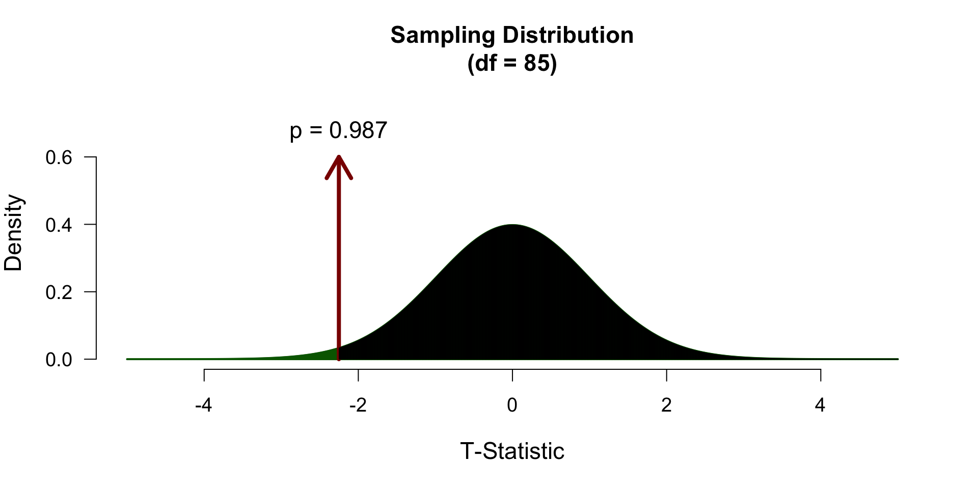
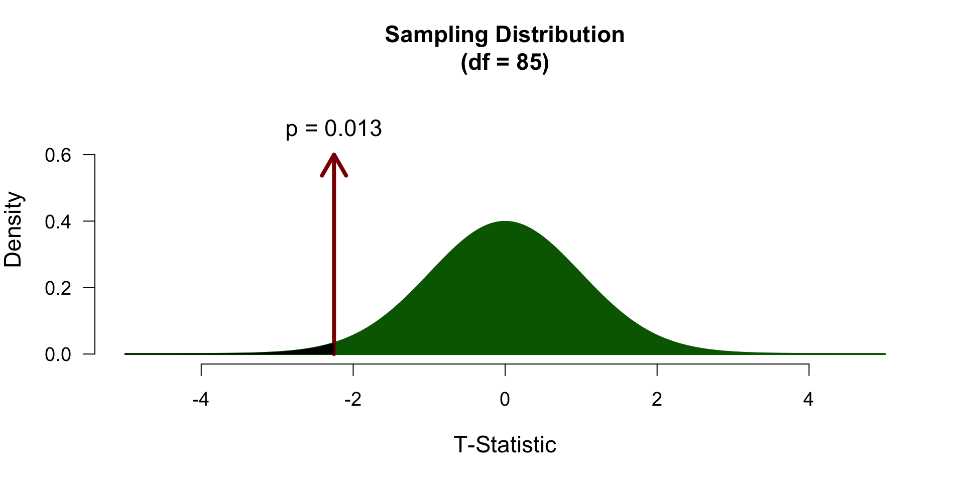
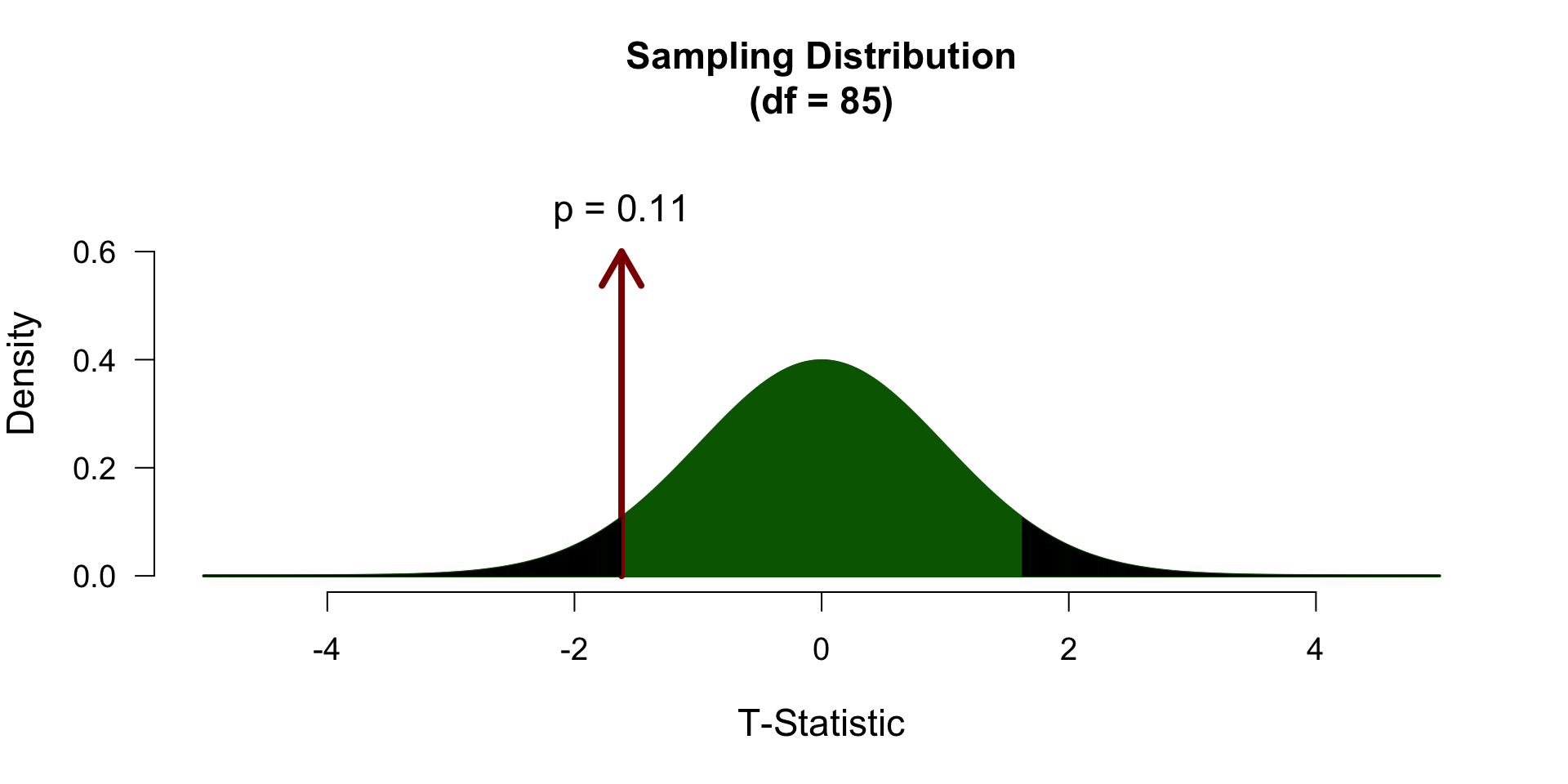
To determine if this t-value significantly differs from the population mean we have to specify a type I error that we are willing to make.
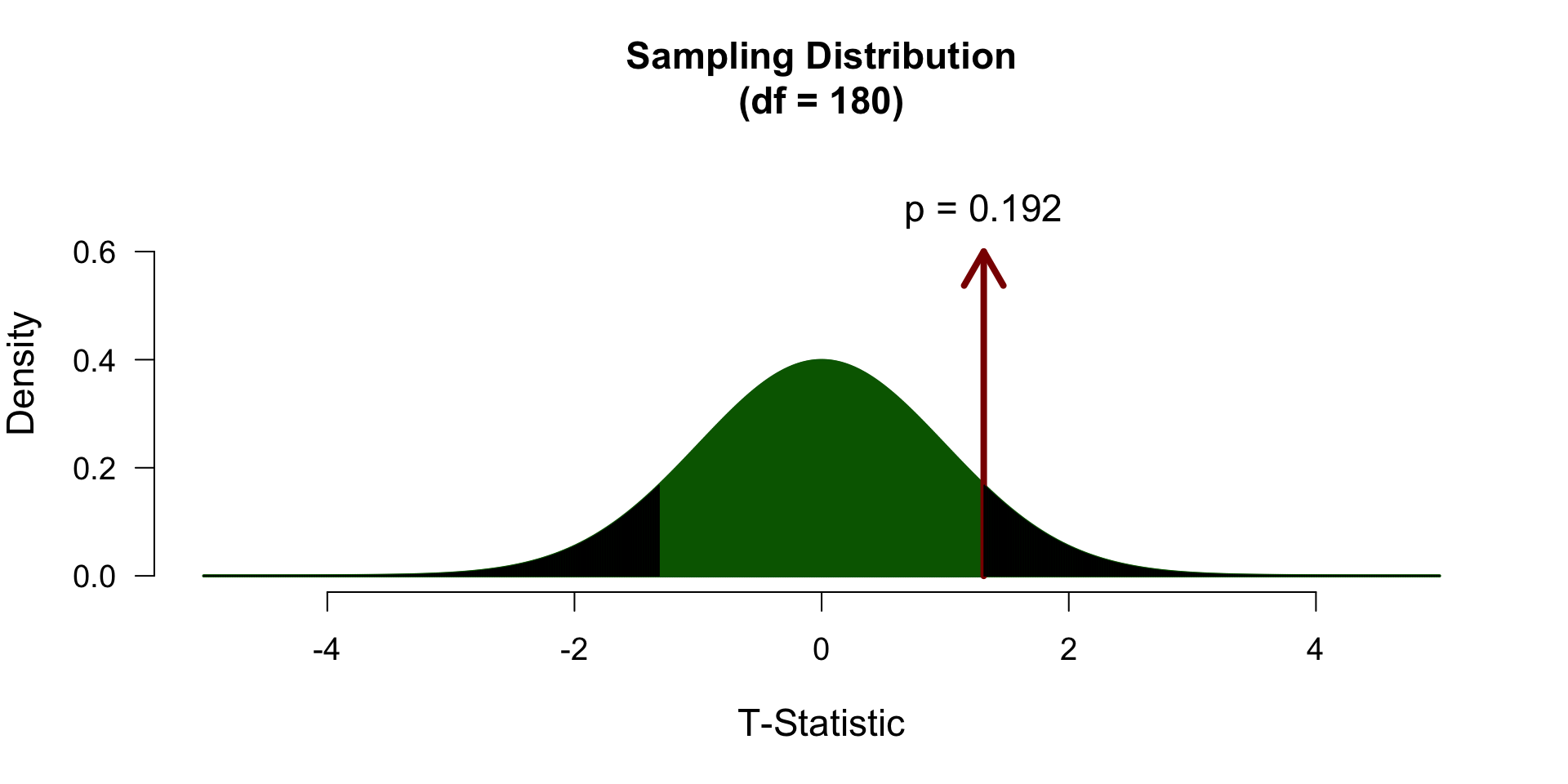
Finally we have to calculate our \(p\)-value for which we need the degrees of freedom \(df = n - 1\) to determine the shape of the t-distribution.
\[ H_A: \mu \neq 120 \rightarrow t \neq 0 \]
\[ H_A: \mu > 120 \rightarrow t > 0 \]
\[ H_A: \mu < 120 \rightarrow t < 0 \]
\[d = \frac{t}{\sqrt{n}}\]
Cohen (1988)
See Tukey (1969) and Section 3.7.4 of Field:
being so disinterested in our variables that we do not care about their units can hardly be desirable.
Compare 2 dependent/paired group means
In the Paired samples t-test the deviation (\(D\)) for each pair is calculated and the mean of these deviations (\(\bar{D}\)) is tested against the null hypothesis where \(\mu = 0\).
\[t_{n-1} = \frac{\bar{D} - \mu}{ {SE}_D }\] Where \(n\) (the number of cases) minus \(1\), are the degrees of freedom \(df = n - 1\) and \(SE_D\) is the standard error of \(D\), defined as \(s_D/\sqrt{n}\).
\[\LARGE{ \begin{aligned} H_0 &: \bar{D} = \mu_D \\ H_A &: \bar{D} \neq \mu_D \\ H_A &: \bar{D} > \mu_D \\ H_A &: \bar{D} < \mu_D \\ \end{aligned}}\]
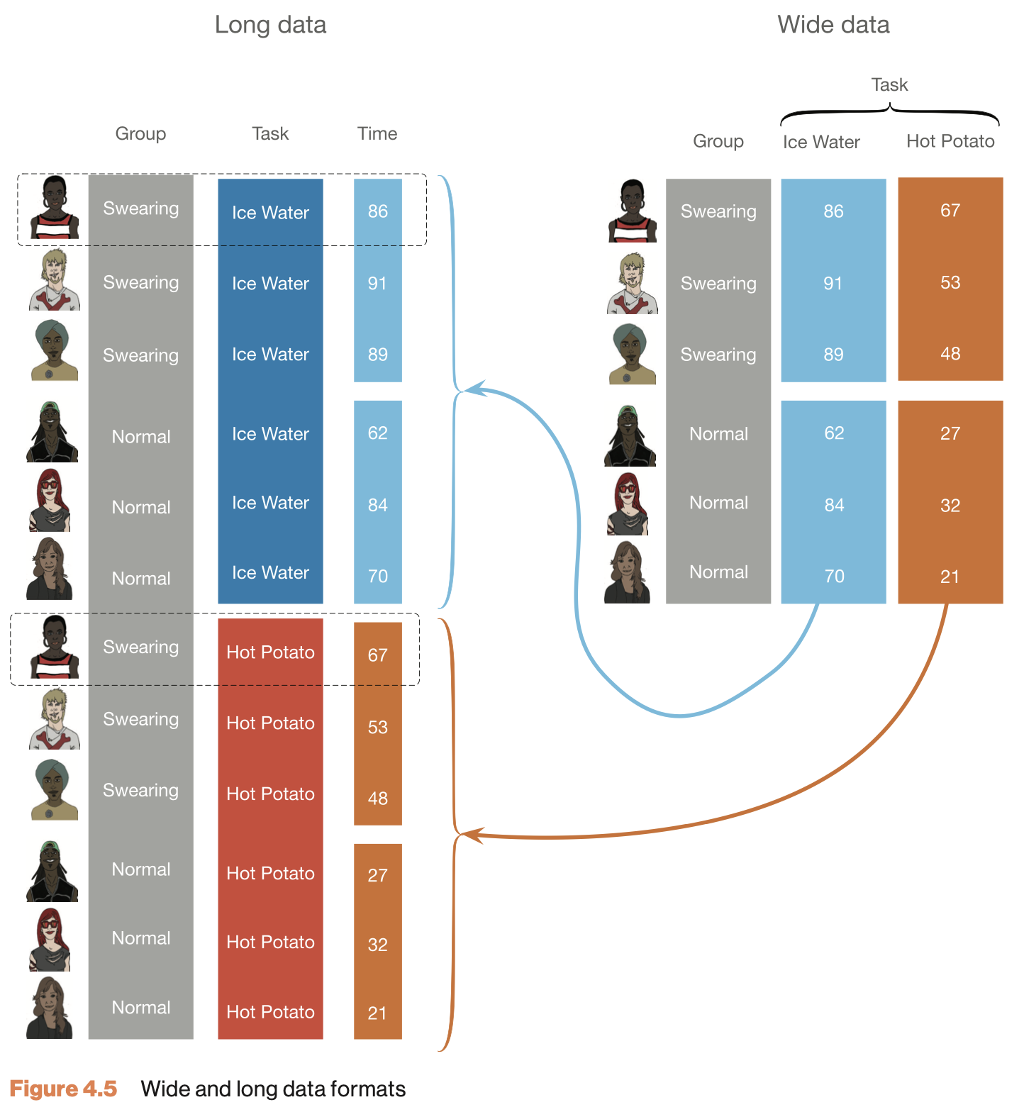
| index | k1 | k2 |
|---|---|---|
| 1 | x | x |
| 2 | x | x |
| 3 | x | x |
| 4 | x | x |
Where \(k\) is the level of the categorical predictor variable and \(x\) is the value of the outcome/dependent variable.
We are going to use the IQ estimates we collected. You had to guess your neighbor’s IQ and your own IQ.
Let’s take a look at the data.
diffScores      <- na.omit(diffScores) # get rid of all missing values
diffMean        <- mean(diffScores)
diffMean
[1] -7.023256And we also need n.
\[t_{n-1} = \frac{\bar{D} - \mu}{ {SE}_D }\]
\[ \mathcal{H}_A: \mu_D \neq 0 \rightarrow t \neq 0 \]
\[d = \frac{t}{\sqrt{n}}\]
Compare 2 independent group means
In the independent-samples t-test the mean of both independent samples is calculated and the difference of these \((\bar{X}_1 - \bar{X}_2)\) means is tested against the null hypothesis where \(\mu = 0\).
\[t_{n_1 + n_2 -2} = \frac{(\bar{X}_1 - \bar{X}_2) - \mu}{{SE}_p}\] Where \(n_1\) and \(n_2\) are the number of cases in each group and \(SE_p\) is the pooled standard error.
| index | k | outcome |
|---|---|---|
| 1 | 1 | x |
| 2 | 1 | x |
| 3 | 2 | x |
| 4 | 2 | x |
Where \(k\) is the level of the categorical predictor variable and \(x\) is the value of the outcome/dependent variable.
Specific for independent sample \(t\)-test:
We are going to use the IQ estimates we collected. You had to guess the IQ of the one sitting next to you and your own IQ. Do your guesses differ from the guesses from last year??
iqLastYear.var <- var(iqLastYear, na.rm = TRUE)
iqThisYear.var <- var(iqThisYear, na.rm = TRUE)
print(rbind(iqLastYear.var, iqThisYear.var))
[,1]
iqLastYear.var 389.3867
iqThisYear.var 779.3506iqLastYear.n <- length(iqLastYear)
iqThisYear.n <- length(iqThisYear)
n <- iqLastYear.n + iqThisYear.n
print(rbind(iqLastYear.n, iqThisYear.n)) [,1]
iqLastYear.n 96
iqThisYear.n 86\[t_{n_1 + n_2 -2} = \frac{(\bar{X}_1 - \bar{X}_2) - \mu}{{SE}_p}\]
Where \({SE}_p\) is the pooled standard error.
\[{SE}_p = \sqrt{\frac{S^2_p}{n_1}+\frac{S^2_p}{n_2}}\]
And \(S^2_p\) is the pooled variance.
\[S^2_p = \frac{(n_1-1)s^2_1+(n_2-1)s^2_2}{n_1+n_2-2}\]
Where \(s^2\) is the variance and \(n\) the sample size.
\[S^2_p = \frac{(n_1-1)s^2_1+(n_2-1)s^2_2}{n_1+n_2-2}\]
\[ {SE}_p = \sqrt{\frac{S^2_p}{n_1}+\frac{S^2_p}{n_2}} \]
\[t_{n_1 + n_2 -2} = \frac{(\bar{X}_1 - \bar{X}_2) - \mu}{{SE}_p}\]
\[ \mathcal{H}_A: \mu_1 \neq \mu_2 \rightarrow t \neq 0 \]
\[d = \frac{2t}{\sqrt{n_1 + n_2}}\]
There exist different hypothesis tests for this - the most used is Levene’s test:
Levene's Test for Homogeneity of Variance (center = median)
       Df F value  Pr(>F)
group   1  2.8824 0.09128 .
      180
---
Signif. codes:  0 '***' 0.001 '**' 0.01 '*' 0.05 '.' 0.1 ' ' 1
But more nuance lies in comparing observed sd’s or variances:
    2025     2026
19.73288 27.91685 Warning
Levene’s test (and other significance tests like it, such as Shapiro for normality) are heavily influenced by sample size, so a significant test result does not necessarily mean that you have a problem. A more pragmatic rule of thumb is to look at the ratio of variances - a ratio greater than 2 is problematic. Additionally, Welch \(t\)-test is a version of the \(t\)-test that is robust to unequal variances.
Unequal variances bias the sampling distribution of \(t\). Welch makes a correction:
\[SE_{\text{unpooled}} = \sqrt{\frac{s_1^2}{n_1} + \frac{s_2^2}{n_2}}\]

Warning
Assumption violations affect the shape of the sampling distribution and mess up the type 1/2 error rates
Board & Fritzon (2005): You don’t have to be ‘mad’ to work here, but it helps
Do managers score higher on histrionic personality disorder than legally classified psychopaths?
Group: 39 managers vs. 317 legally classified psychopathsHistrionic personality index: MMPI-PD scoreTuk et al. (2011): Bladder control
Are people with full bladders inhibited more than those without?
urgency: drink all five cups of water vs. take a sip from eachll_sum: number of trials (out of 8) choosing a large, later reward over a small, sooner oneGelman & Weakliem (2009): The beautiful people
Do the most beautiful celebrities (People magazine, 1995–2000) have more daughters than sons?
daughters: number of daughters, as of 2007sons: number of sons, as of 2007

Scientific & Statistical Reasoning