20. Non-parametric tests

Author

Affiliation

Johnny van Doorn

University of Amsterdam

Published

20 October 2026

In this lecture we aim to:

Repeat some assumptions
Introduce rank-based methods
Look at rank-based equivalents to some old friends
Show these in JASP

Reading: Chapter 15 (§15.1–15.9)

Nonparametric tests

When assumptions are violated
- e.g., strong non-normality
When the variable is ordinal
- e.g., when playing Mario Kart
When unsure about outliers
- e.g., some observations with z \(\approx\) 3
Topic of my dissertation!

I’m Ken Griffey on the Mariners
Okay, I’m way beyond the boundaries, outside of parameters
The rap chancellor, jacket made of camel fur

Mac Miller, Apparition (Faces)

Parametric vs Nonparametric

Attribute	Parametric	Nonparametric
distribution	normally distributed	any distribution
sampling	random sample	random sample
sensitivity to outliers	yes	no
works with	large data sets	small and large data sets
speed	fast	slow

Ranking

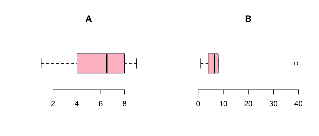
A	1	4	6	7	8	9
B	1	4	6	7	8	39
rank(A)	1	2	3	4	5	6
rank(B)	1	2	3	4	5	6

Ties

index	1	2	3	4	5	6	7	8	9
x	11	42	42	62	73	73	84	84	84
ranks	1	2.5	2.5	4	5.5	5.5	8	8	8

\[\frac{2 + 3}{2} = 2.5, \frac{5 + 6}{2} = 5.5, \frac{7 + 8 + 9}{3} = 8\]

Procedure

Assumption: independent random samples.
Hypothesis:
\(H_0\) : equal population distributions (implies equal mean ranking)
\(H_A\) : unequal mean ranking (two sided)
\(H_A\) : higher mean ranking for one group.
Test statistic is difference between mean or sum of ranking.
Standardize test statistic to normal sampling distribution.
Calculate P-value one or two sided.
Conclude to reject \(H_0\) if \(p < \alpha\).

What does \(H_0\) state?

Test	\(H_0\)
Wilcoxon rank-sum (Mann-Whitney)	Both groups come from the same population distribution
Wilcoxon signed-rank	Positive and negative differences are equally likely (symmetric around 0)
Kruskal-Wallis	All groups come from the same population distribution
Friedman’s ANOVA	Within each participant, every order of the conditions is equally likely

Under \(H_0\) the mean ranks are equal; rejecting it means one group or condition tends to score higher
Not a test of means, and of medians only if the distributions have the same shape

Wilcoxon rank-sum test

Independent 2 samples

Also known as the Mann-Whitney U test

Wilcoxon rank-sum test

Developed by Frank Wilcoxon the rank-sum test is an nonparametric alternative to the independent samples t-test.

By ranking all values and then summing the ranks per group, one would expect under the null hypothesis, that the sum of ranks is approximately equal.

After standardizing the test statistic (summed ranks for one group), we can use the standard normal distribution as the sampling distribution.

Example

Data (.jasp) · Results (.jasp) · Results (.html)

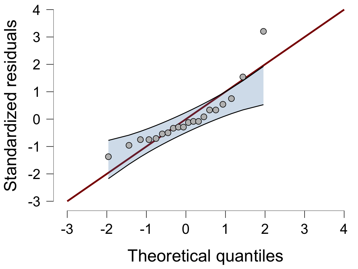
Q-Q plot of the residuals

Sunday BDI, independent \(t\)-test in JASP: Assumption Checks → Q-Q plot residuals → Confidence interval¹

More on this in the extra text on skewed data (Student, Welch or Mann-Whitney?)

Test statistic W is the sum of ranks per group

rankSums <- aggregate(rankedBDI ~ Drug, data, sum)
rankSums

     Drug rankedBDI
1 Alcohol      90.5
2 Ecstasy     119.5

We can take the sum of ranks for the first group as W:

W <- rankSums[1, 2]
W

[1] 90.5

Subtracting the minimum score

JASP reports the value of U, which is W with its minimum value subtracted:

W.min <- sum(1:10); W.min

[1] 55

U <- W - W.min
U

[1] 35.5

JASP (and the book) take the ecstasy group: 119.5 - 55 = 64.5
The two add up to \(n_1 n_2\) = 100

Normal approximation for W

To calculate the Z-score we need to standardize the W. To do so we need the mean W and the standard error of W.

For this we need the sample sizes for each group.

n <- aggregate(rankedBDI ~ factor, data, length)

n.1 <- n$rankedBDI[1]
n.2 <- n$rankedBDI[2]

cbind(n.1, n.2)

     n.1 n.2
[1,]  10  10

Mean W under \(H_0\)

\[\bar{W}_s=\frac{n_1(n_1+n_2+1)}{2}\]

W.mean <- (n.1 * (n.1 + n.2 + 1)) / 2
W.mean # this is the middle point between the min and max value of W

[1] 105

W.max <- sum(11:20); W.max

[1] 155

W.min <- sum(1:10); W.min

[1] 55

SE W

\[{SE}_{\bar{W}_s}=\sqrt{ \frac{n_1 n_2 (n_1+n_2+1)}{12} }\]

W.se <- sqrt((n.1 * n.2 * (n.1 + n.2 + 1)) / 12)
W.se

[1] 13.22876

Calculate Z

\[z = \frac{W - \bar{W}}{{SE}_W}\]

Which looks a lot like

\[\frac{X - \bar{X}}{{SE}_X} \text{or} \frac{b - \mu_{b}}{{SE}_b} \]

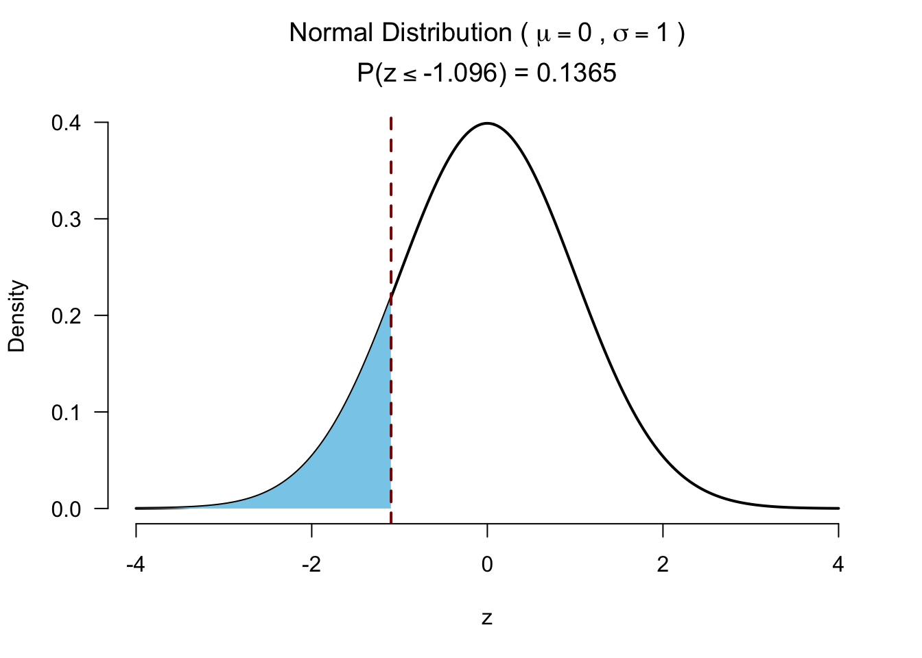
z <- (W - W.mean) / W.se
z

[1] -1.096097

Test for significance 2 sided

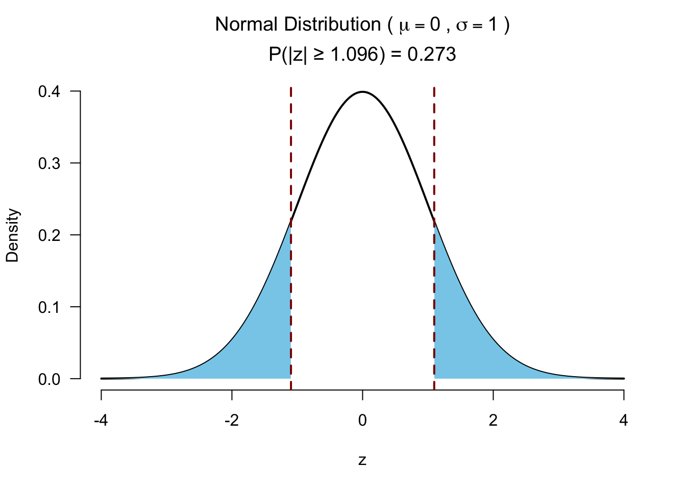
JASP: U = 64.5, p = .286, a bit higher because of a continuity correction (Jane Superbrain 15.2)

Test for significance 1 sided

Effect size rank-biserial correlation

\[r_{bs} = 1 - \frac{2*W}{n_1*n_2}\]

W <- W - W.min # use modern W
biserialCor <- 1 - (2*(W)) / (n.1*n.2);
biserialCor

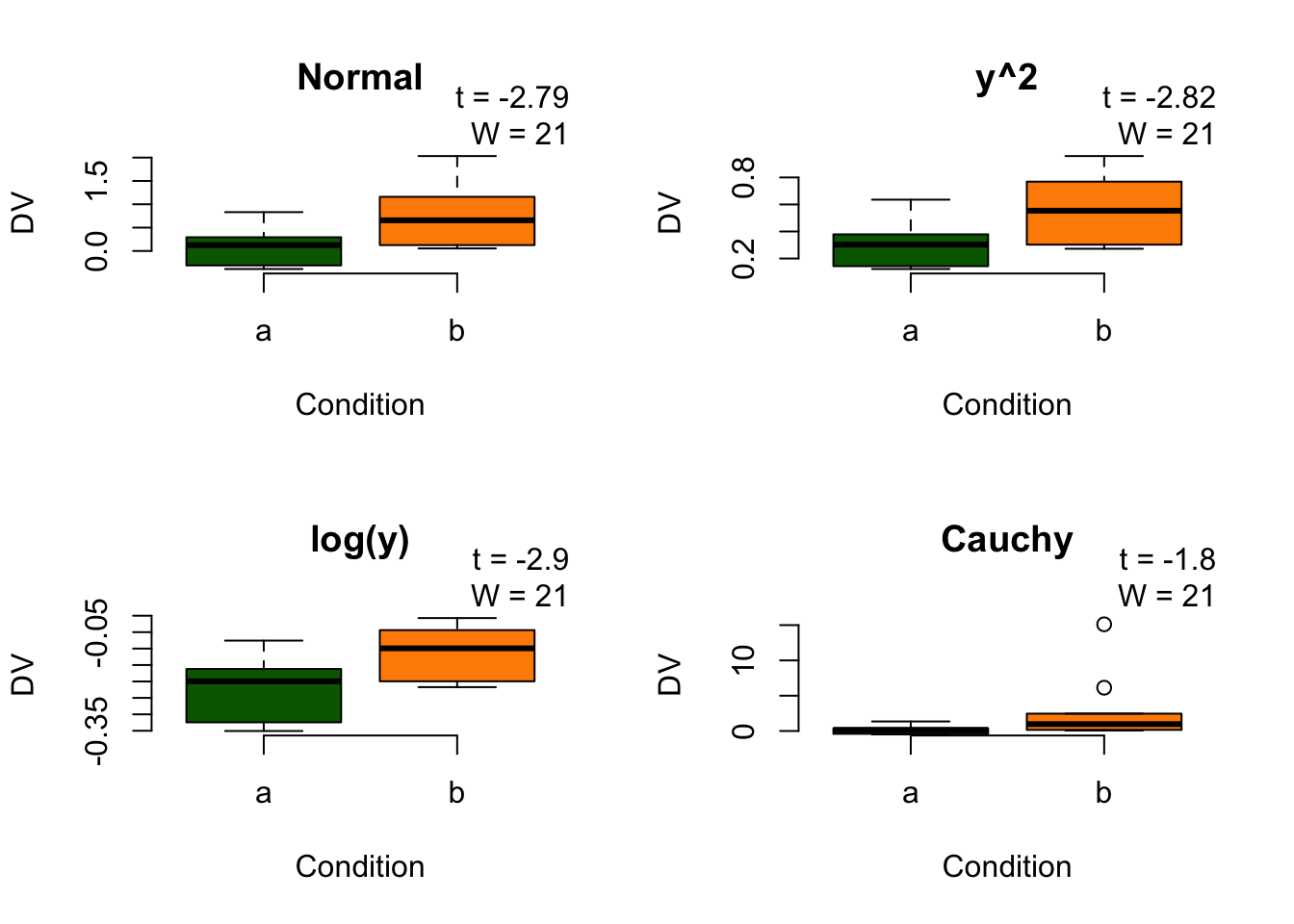
[1] 0.29

Robustness under monotonic transformations

Wilcoxon signed-rank test

Paired 2 samples

Wilcoxon signed-rank test

The Wilcoxon signed-rank test is a nonparametric alternative to the paired samples t-test. It assigns + or - signs to the difference between two repeated measures. By ranking the absolute differences and summing these ranks for the positive group, the null hypothesis is tested that positive and negative differences are equally likely.

Example

Data (.jasp) · Results (.jasp) · Results (.html)

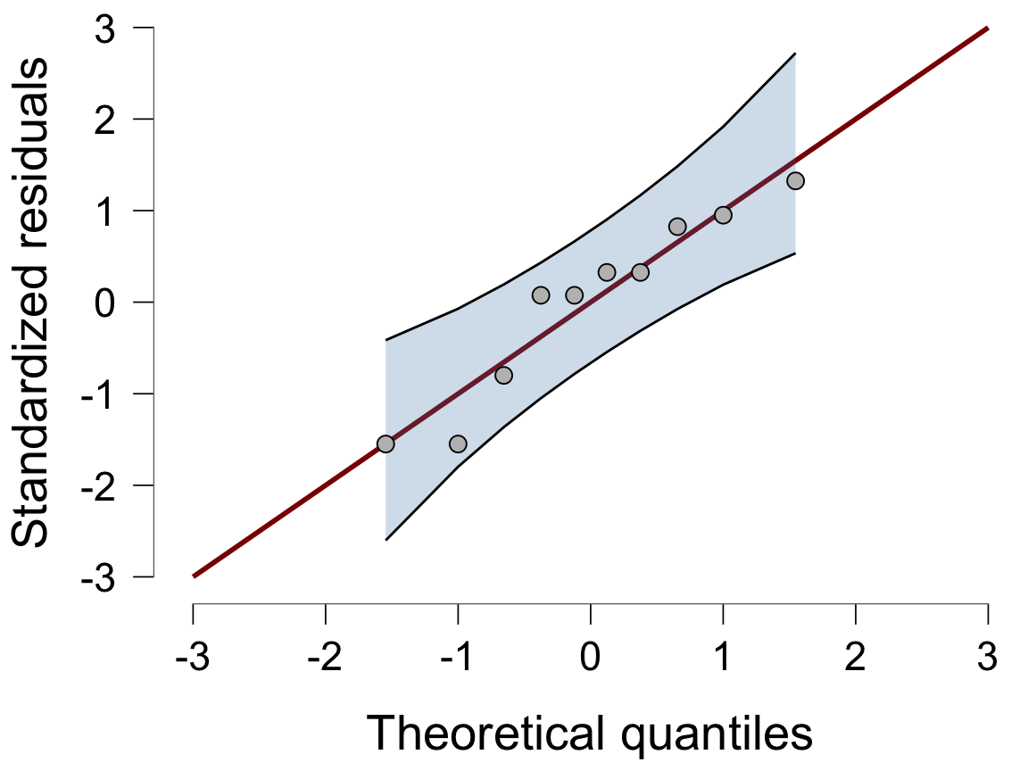
Q-Q plot of the differences

Paired samples \(t\)-test in JASP: Assumption Checks → Q-Q plot residuals → Confidence interval

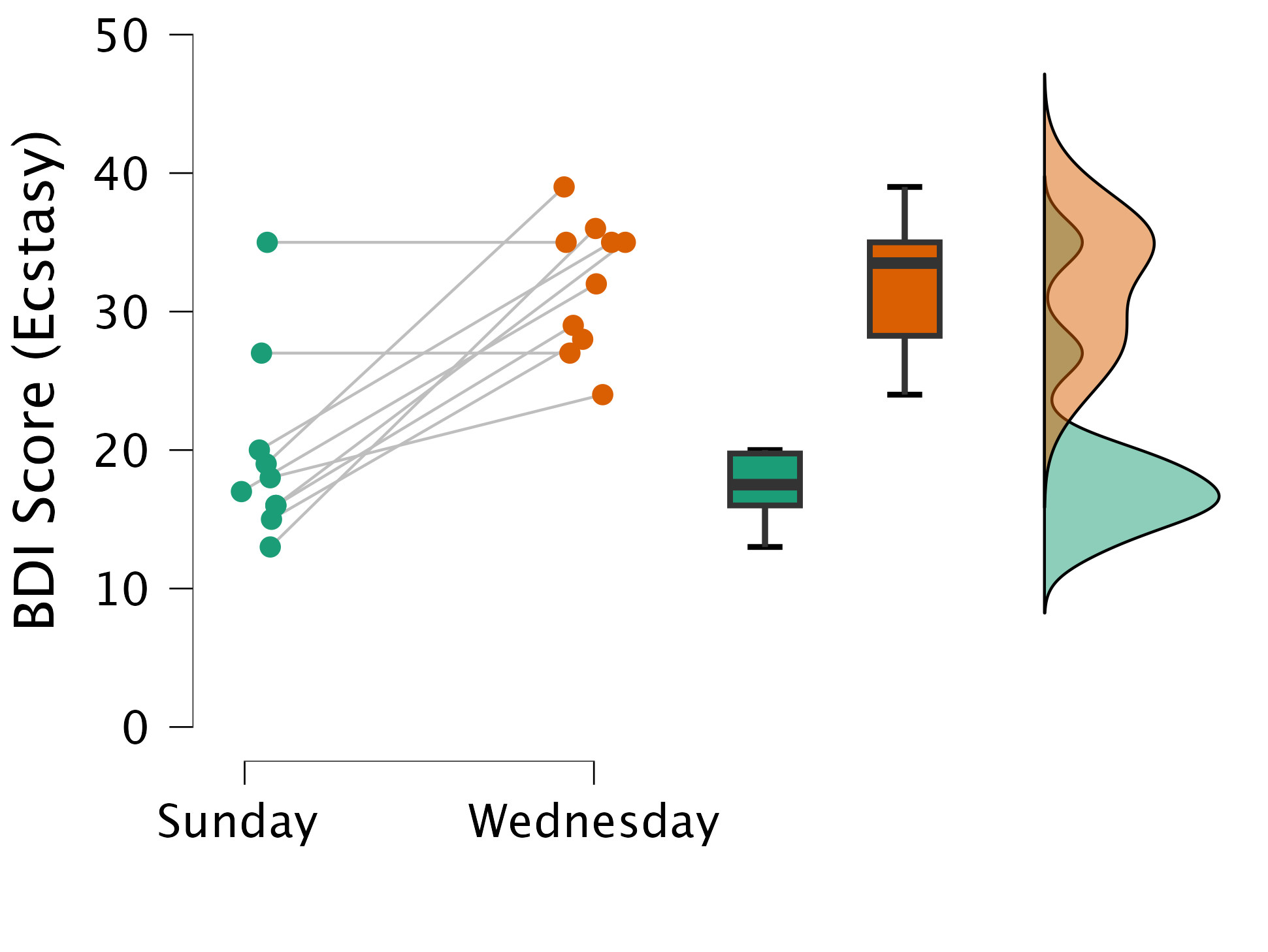
The plot

Calculate T

# Calculate difference in scores between second and first measure (as in the book)
data$diff = data$Wednesday - data$Sunday

# Calculate absolute difference in scores between second and first measure
data$abs.diff = abs(data$Wednesday - data$Sunday)

# Remove observations where the difference is 0
data <- data[data$diff != 0, ]

# Create rank variable
data$rank <- rank(data$abs.diff)

# Assign a '+' or a '-' to those values 
data$sign <- sign(data$Wednesday - data$Sunday)

The data

Data (.jasp) · Results (.jasp) · Results (.html)

Calculate \(T_+\)

# Calculate the sum of the positive ranks
T_pos <- sum(data$rank * (data$diff > 0))
T_pos

[1] 36

# Calculate N without 0 (no differences).
n <- nrow(data)
n

[1] 8

How likely is it to observe the highest possible rank sum (36), for \(n=8\), if there is no difference in BDI between Sunday and Wednesday?

Calculate \(\bar{T}\) and \({SE}_{T}\)

\[\bar{T} = \frac{n(n+1)}{4}\]

T_mean <- (n*(n+1))/4
T_mean

[1] 18

T_mean is the middle point between the minimum (0) and maximum possible (36) value for T

\[{SE}_{T} = \sqrt{\frac{n(n+1)(2n+1)}{24}}\]

SE_T <- sqrt( (n*(n+1)*(2*n+1)) / 24)

Calculate Z

\[z = \frac{T_+ - \bar{T}}{{SE}_T}\]

z <- (T_pos - T_mean)/SE_T
z

[1] 2.520504

Test for significance

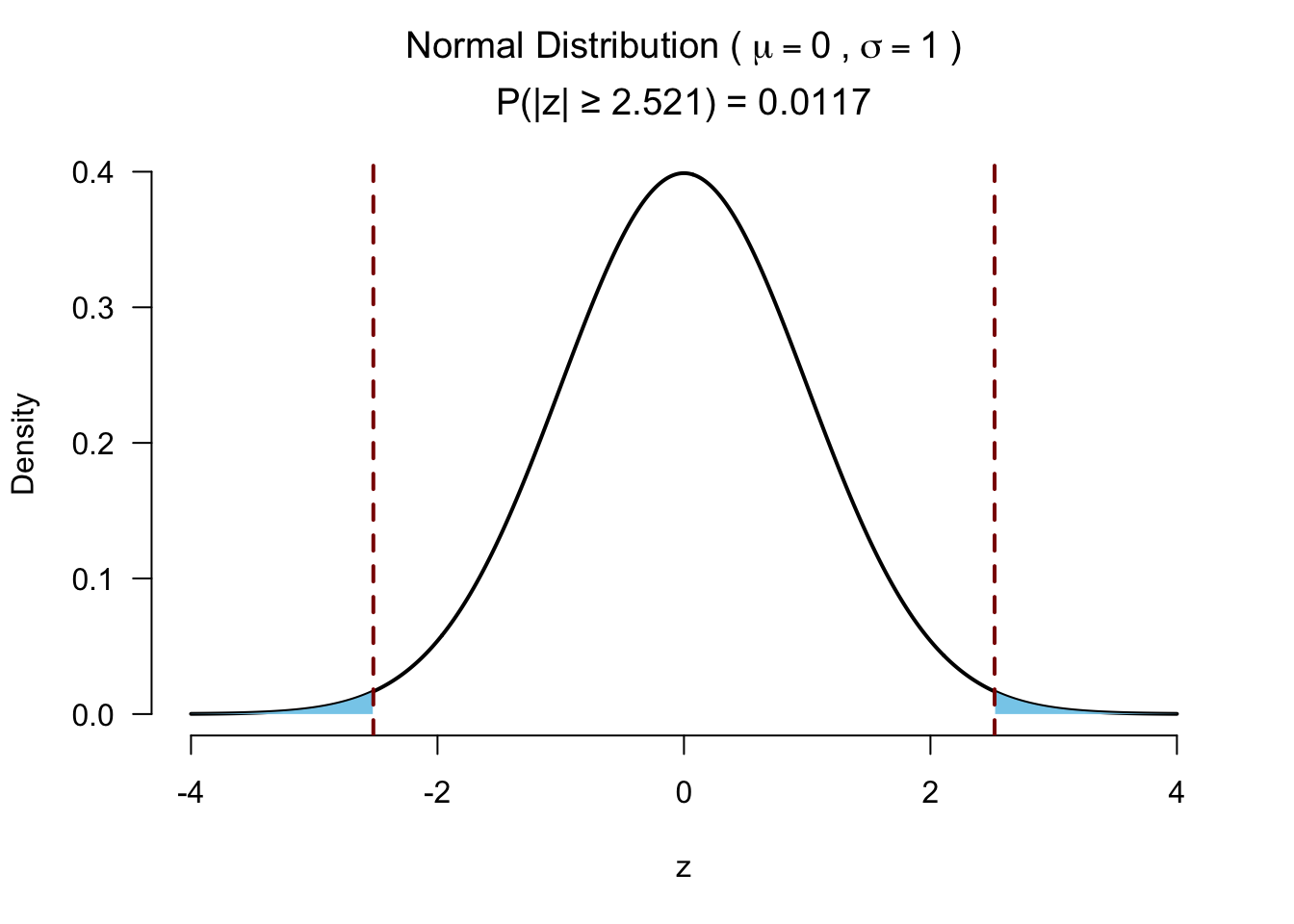
JASP: W = 36, p = .014, a bit higher because of a continuity correction (Jane Superbrain 15.2)

Effect size

Matched rank-biserial correlation

\[r = \frac{T_+ - T_- }{T_+ + T_-}\]

Here \(T_+\) is the sum of the positive ranks (i.e., where Wednesday > Sunday), which is 36. \(T_-\) is the sum of the negative ranks, which do not exist. We have a maximum positive correlation (i.e., everybody with a difference scored higher on Wednesday).

T_neg <- sum(data$rank * (data$diff < 0)) # sum negative ranks
T_neg

[1] 0

rbis <- (T_pos - T_neg) / (T_pos + T_neg)
rbis

[1] 1

Kruskal–Wallis test

Independent >2 samples

Kruskal–Wallis test

Created by William Henry Kruskal and Wilson Allen Wallis, the Kruskal-Wallis test is a nonparametric alternative to the independent one-way ANOVA.

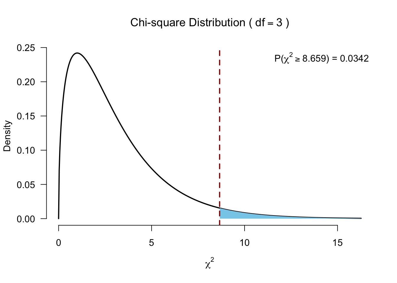
The Kruskal-Wallis test essentially subtracts the expected mean ranking from each observed mean ranking, which is \(\chi^2\) distributed.

Assign ranks

# Assign ranks
data$ranks <- rank(data$Testosterone)

The data

Data (.jasp) · Results (.jasp) · Results (.html)

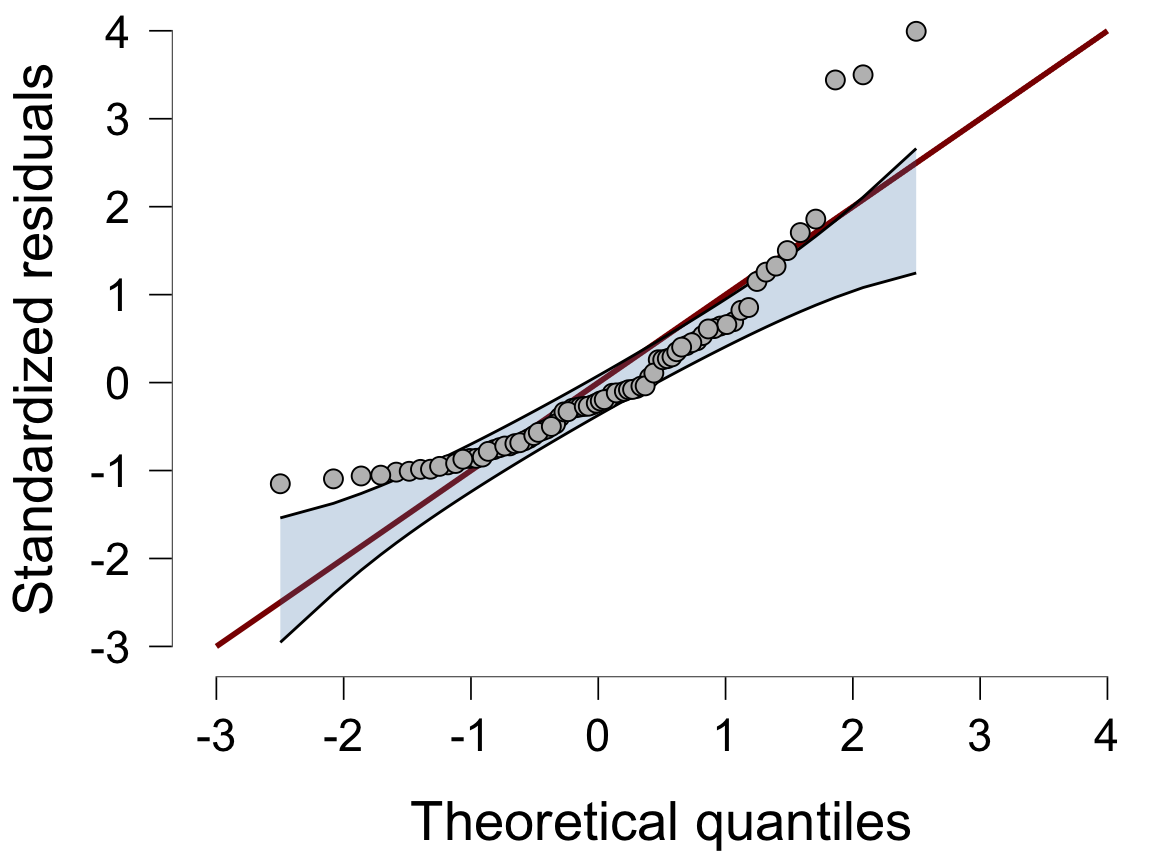
Q-Q plot of the residuals

One-way ANOVA in JASP (as in the book, Figure 15.10)

Calculate H

\[H = \frac{12}{N(N+1)} \sum_{i=1}^k \frac{R_i^2}{n_i} - 3(N+1)\]

\(N\) total sample size
\(n_i\) sample size per group
\(k\) number of groups
\(R_i\) rank sums per group

Calculate H

# Now we need the sum of the ranks per group.
R.i <- aggregate(ranks ~ Soya, data = data, sum)$ranks
R.i

[1] 883 883 547 927

# De total sample size N is:
N <- nrow(data)

# And the sample size per group is n_i:
n.i <- aggregate(Testosterone ~ Soya, data=data, length)$Testosterone
n.i

[1] 20 20 20 20

Calculate H

\[H = \frac{12}{N(N+1)} \sum_{i=1}^k \frac{R_i^2}{n_i} - 3(N+1)\]

H <- ( 12/(N*(N+1)) ) * sum(R.i^2/n.i) - 3*(N+1)
H

[1] 8.658889

And the degrees of freedom

k  <- 4
df <- k - 1

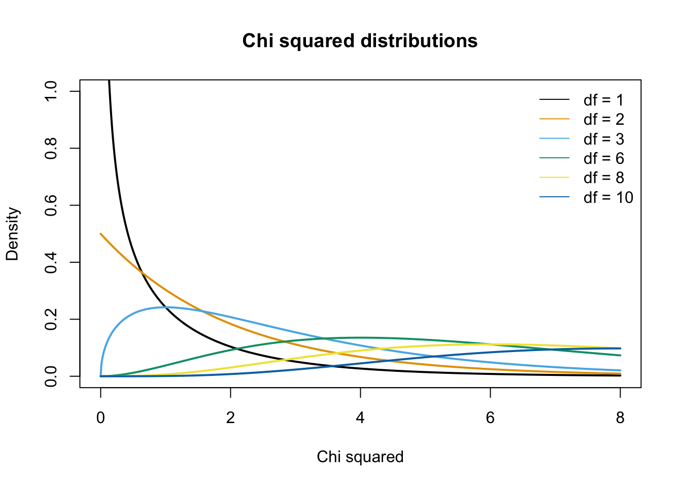
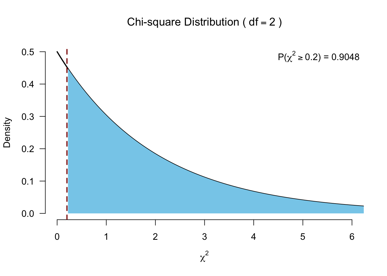
\(\chi^2\) distribution

The \(\chi^2\) distribution describes the test statistic under the assumption of \(H_0\), given the degrees of freedom.

Test for significance

Follow-up?

Dunn’s post hoc test:
- Pairwise Mann-Whitney tests with adjusted p-values

Friedman’s ANOVA

Paired >2 samples

Friedman’s ANOVA

Created by Milton Friedman the Friedman’s ANOVA is a nonparametric alternative to the repeated one-way ANOVA.

Just like the Kruskal-Wallis test, Friedman’s ANOVA, subtracts the expected mean ranking from the calculated observed mean ranking, which is also \(\chi^2\) distributed.

The data

Data (.jasp) · Results (.jasp) · Results (.html)

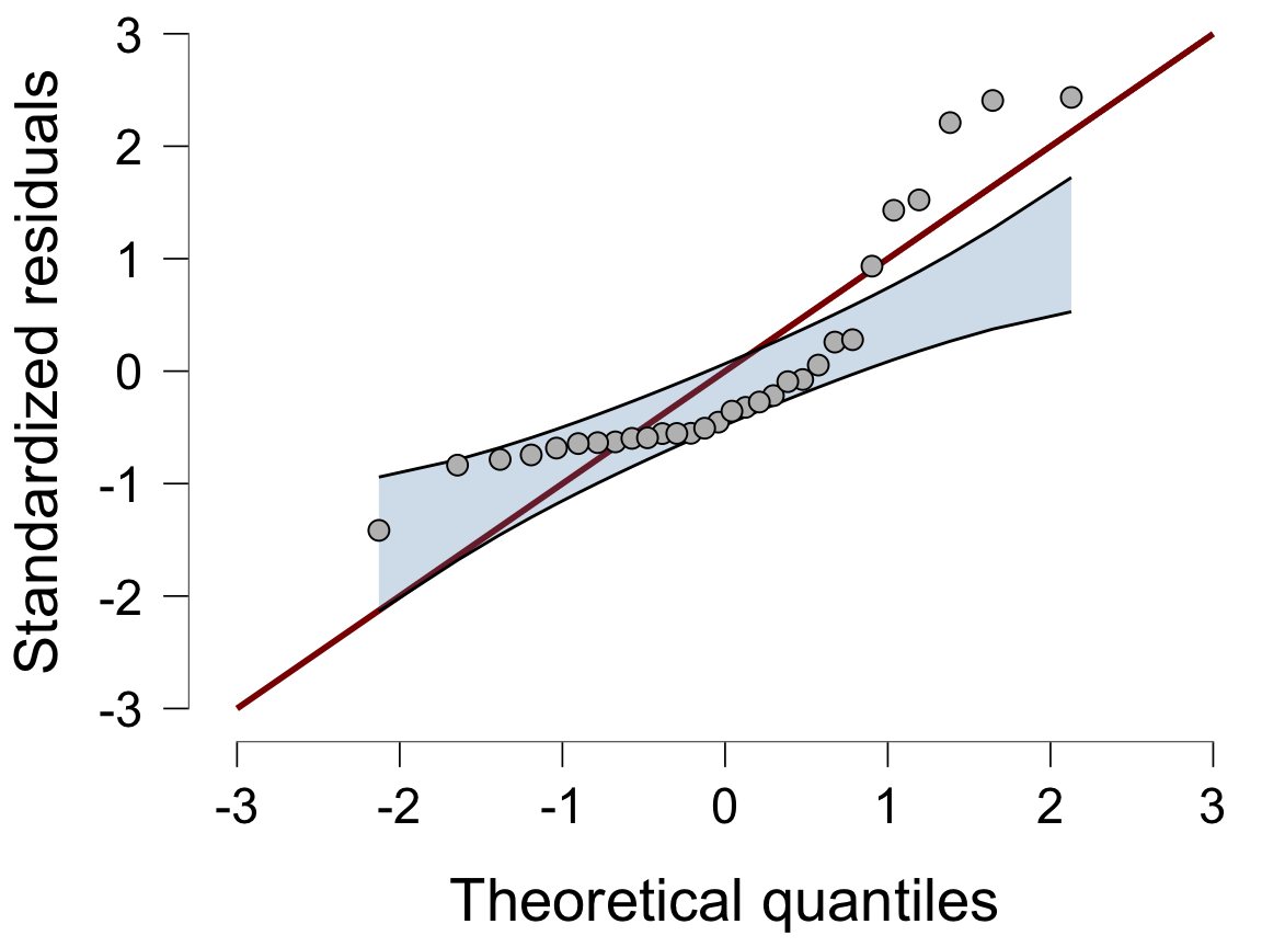
Q-Q plot of the residuals

Repeated measures ANOVA in JASP (as in the book, Figure 15.13)

Assign ranks

Rank within each participant (i.e., within each row).

# Rank for each person
ranks <- t(apply(data, 1, rank))

The data with ranks

Calculate \(F_r\)

\[F_r = \left[ \frac{12}{Nk(k+1)} \sum_{i=1}^k R_i^2 \right] - 3N(k+1)\]

\(N\) total number of subjects
\(k\) number of groups
\(R_i\) rank sums for each group

–> We sum the ranks for each of the three experimental conditions (and apply some standardizations).

Calculate \(F_r\) (without adjusting for ties)

Calculate ranks sum per condition and \(N\).

R.i <- apply(ranks, 2, sum)
R.i

 Start_R Month1_R Month2_R 
      19       20       21

# N is number of participants
N <- 10

k <- 3
F.r <- ( ( 12/(N*k*(k+1)) ) * sum(R.i^2) ) - ( 3*N*(k+1) )
F.r

[1] 0.2

Adjusting for ties (just for fun)

\[ \frac{(k-1) \sum_i^k (R_i - \frac{b(k+1))}{2})^2}{\sum_i^b \sum_j^k (R_{ij}^2) - \frac{bk(k+1)^2}{4}} \]

k <- 3
b <- 10
F.r <- (sum ((R.i - ((b*(k+1))/2) )^2) * (k-1)) / (sum((ranks^2)) - (b*k *(k+1)^2) / 4)
F.r

[1] 0.2

And the degrees of freedom

df <- k - 1

Test for significance

Post hoc tests?

Conover test
Follow up with Wilcoxon signed-rank tests!

JASP

Closing

Recap

Non-parametric tests are rank-based, which means they are robust to:
- Non-normality
- Transformations of the data
- Outliers

Recap lecture 18

Accidents in a driving simulator, for every combination of alcohol and speed

pp, participant number
Daytime, morning or evening
none_alc_none_speed to much_alc_much_speed, accidents in each of the 9 combinations

Data (.csv) · Results (.jasp) · Results (.html)

Recap lecture 18: \(t\)-test = ANOVA = regression

The same pre- and posttest scores, analyzed in two ways

Ignoring participants, independent \(t\)-test = one-way ANOVA = regression
Accounting for participants, paired \(t\)-test = RM ANOVA = ANOVA or regression with id
y, id and time-point, long format (one row per measurement)
pre-test, post-test and diff-scores, wide format (one row per participant)

Data (.csv) · Results (.jasp) · Results (.html)

Exam note: assumptions per analysis

All analyses below assume normal residuals (Q-Q plot with confidence band)
Violations (normality, variances, sphericity) mess up Type I/II error rates
How to assess them (next slides)

Analysis	Also assumes	If unequal variances or no sphericity	If non-normal
Paired \(t\)-test	–	–	Wilcoxon signed-rank
Independent \(t\)-test	Equal variances	Welch \(t\)	Mann-Whitney
One-way ANOVA	Equal variances	Welch \(F\)	Kruskal-Wallis
Factorial ANOVA	Equal variances	–	–
ANCOVA	Equal variances, independent covariate, equal slopes	–	–
RM ANOVA	Sphericity (3+ levels)	Greenhouse-Geisser	Friedman (one-way only)
Mixed ANOVA	Equal variances, sphericity	Greenhouse-Geisser	–

Exam note: checking assumptions

What you should know: how to assess, robust alternatives, and why these assumptions matter

No assumption NHST (Shapiro-Wilk, Levene’s) on the exam (see Jane Superbrain Box 6.7)
Normality: Q-Q plot of the residuals, with confidence interval
- Assumption Checks → Q-Q plot residuals → Confidence interval
- Points outside the band suggest non-normality
Equal variances: ratio of the largest to the smallest variance (Section 6.9.6)
- Ratio of 2 or more suggests unequal variances
- Equivalently for sd’s: ratio of \(\sqrt{2} \approx 1.4\) or more

Exam note: robust alternatives

Unequal variances:
- Welch \(t\)-test
- Welch \(F\) (one-way ANOVA only: Assumption Checks → Homogeneity corrections)
Non-normality: nonparametric test (Chapter 15; lecture 20)
- Mann-Whitney, Wilcoxon signed-rank, Kruskal-Wallis, Friedman
Question can give a decision rule, e.g., “use nonparametric test if more than 5 points fall outside the Q-Q confidence band”
ANCOVA: no robust version, so have to eat the grain of salt if normality or variances seem problematic

Exam note: ANCOVA assumptions

Independence of the covariate and treatment effect
- ANOVA with the covariate as dependent variable
- What it means: groups differ on the covariate
Homogeneity of regression slopes: interaction covariate * independent variable
- Model → Model Terms: add or remove the interaction
- What it means: effect of the covariate differs between groups

Exam note: lectures 17 and 18

Post hoc tests (lecture 17)
- Know where the options are, exam question will inform you which correction to use
RM ANOVA (lecture 18)
- No sums of squares or effect size calculations required for the exam

Next Time

Multiple regression (lecture 21)

Recommended Exercises

Labcoat Leni 15.1

Matthews et al. (2007): Having a quail of a time?

Do males fertilize more eggs when mating in the context that signalled a mating opportunity?

signalled: eggs fertilized in the male’s signalled context
control: eggs fertilized in the male’s control context
Both males mated with the same 14 females

Data (.jasp) · Results (.jasp) · Results (.html)

Labcoat Leni 15.2

Çetinkaya & Domjan (2006): Eggs-traordinary

Do fetishistic quail fertilize more eggs and initiate sex more quickly?

groups: fetishistic, non-fetishistic or control
egg_percent: percentage of eggs fertilized
latency: time taken to initiate copulation

Data (.jasp) · Results (.jasp) · Results (.html)

Contact

Footnotes

The book (Figure 15.4) checks the raw scores per group, with separate Q-Q plots from the Descriptives module. Its Q-Q plots (also Figures 15.10 and 15.13) have no confidence band, which JASP added later.↩︎