26. Moderation

Author

Affiliation

Johnny van Doorn

University of Amsterdam

Published

6 November 2026

In this lecture we aim to:

Look at interactions between continuous predictors
Revisit the Process module
Demonstrate in JASP

Reading: Chapter 10 (§10.1–10.3)

Moderation

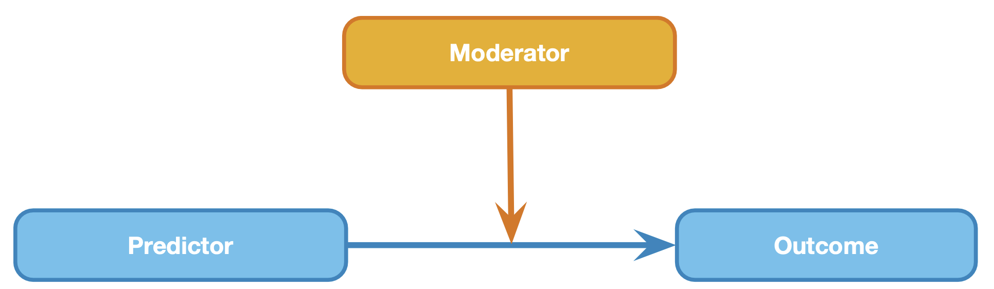
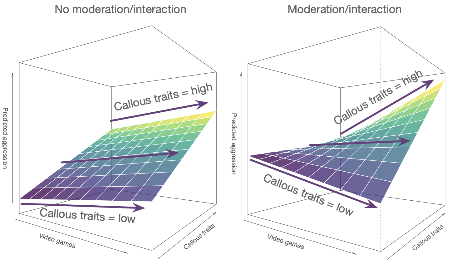
In statistics and regression analysis, moderation occurs when the relationship between two variables depends on a third variable. The third variable is referred to as the moderator variable or simply the moderator. The effect of a moderating variable is characterized statistically as an interaction.

Source WIKIPEDIA

Model

\(\definecolor{red}{RGB}{255,0,0} \definecolor{black}{RGB}{0,0,0} \color{black}Out_i = b_0 + b_1 Pred_i + b_2 Mod_i + \color{red}b_3 Pred_i \times Mod_i \color{black}+ \epsilon_i\)

Model

Assumptions

A selection from Field (8.3 Bias in linear models):

For simple regression

Sensitivity
Homoscedasticity
- See here for further illustration
Linearity
Normality

Additionally, for multiple regression

Multicollinearity (Section 8.9)

View data

Model

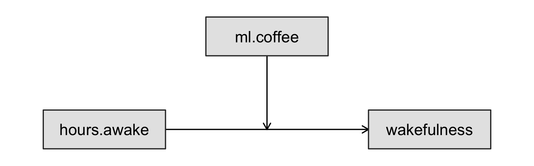
\[\definecolor{red}{RGB}{255,0,0} \definecolor{black}{RGB}{0,0,0} \begin{aligned} \color{black}\text{wakefulness}_i = {} & b_0 + b_1\,\text{hours.awake}_i + b_2\,\text{ml.coffee}_i \\ & + \color{red}b_3\,\text{hours.awake}_i \times \text{ml.coffee}_i \color{black}+ \epsilon_i \end{aligned}\]

Correlations

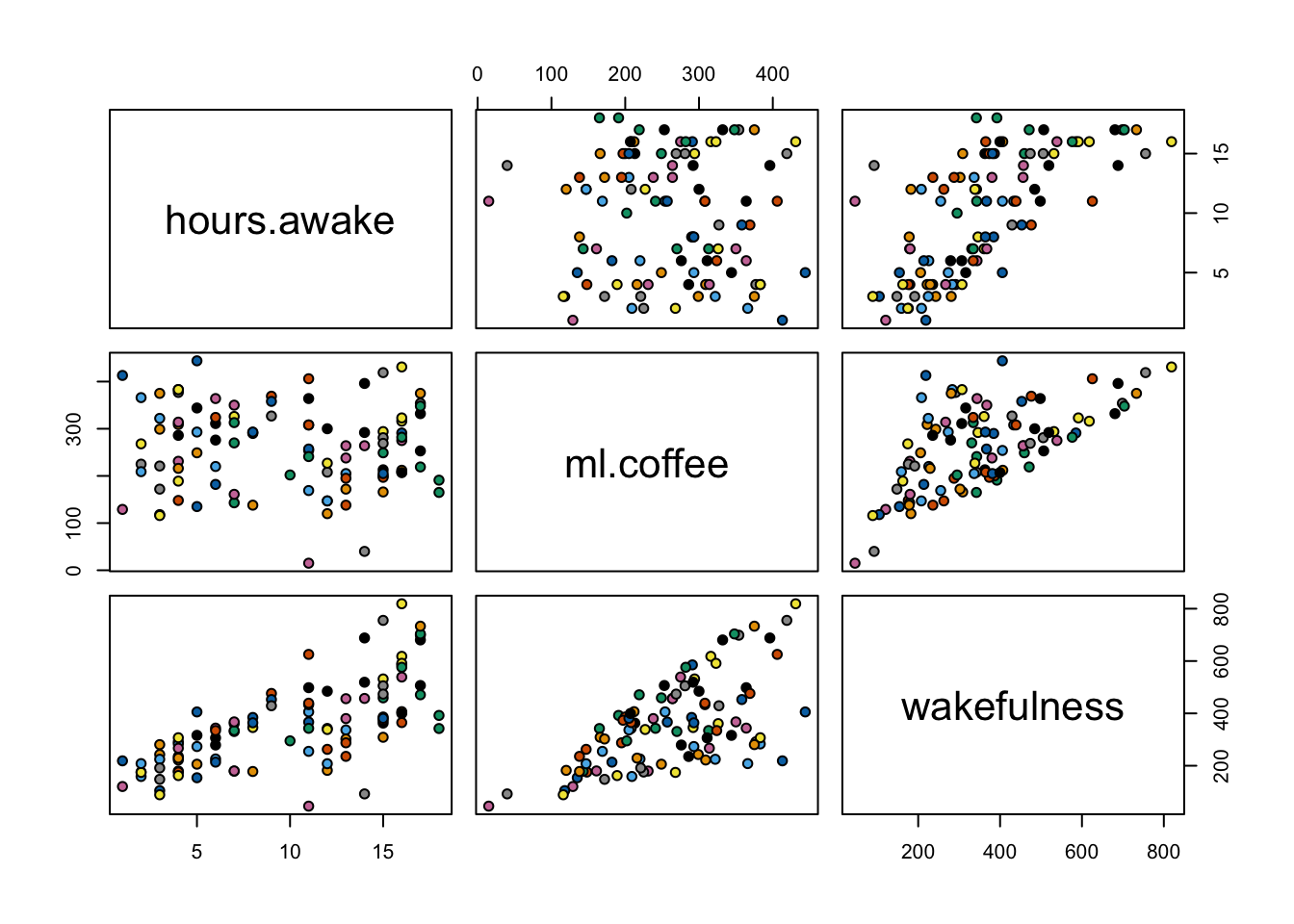
cor(data)

            hours.awake   ml.coffee wakefulness
hours.awake  1.00000000 -0.05495344   0.6935663
ml.coffee   -0.05495344  1.00000000   0.6175888
wakefulness  0.69356633  0.61758884   1.0000000

Scatterplots

3D plot

Take it for a spin

Descriptives plot

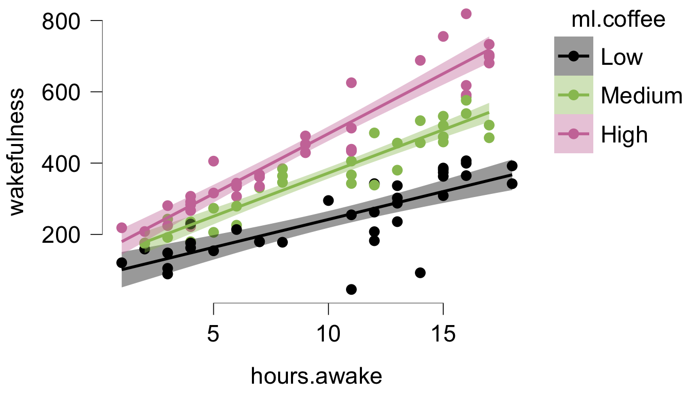
Coffee groups

## Where JASP's descriptives plot splits ml.coffee (default, 3 groups)
round(mean(ml.coffee) + c(-0.5, 0.5) * sd(ml.coffee), 1)

[1] 216.0 303.8

Fit model

fit <- lm(wakefulness ~ hours.awake + ml.coffee + hours.awake*ml.coffee); summary(fit)$coefficients

                        Estimate   Std. Error   t value     Pr(>|t|)
(Intercept)           61.6830508 12.103218305  5.096417 1.732742e-06
hours.awake           -3.6115498  1.123005892 -3.215967 1.772112e-03
ml.coffee              0.2656631  0.042872680  6.196560 1.437213e-08
hours.awake:ml.coffee  0.1024289  0.004037037 25.372290 2.355332e-44

Regression equation

\(\definecolor{red}{RGB}{255,0,0} \definecolor{black}{RGB}{0,0,0} \color{black}\widehat{Out_i} = b_0 + b_1 Pred_i + b_2 Mod_i + \color{red}b_3 Pred_i \times Mod_i \color{black}\)

\(\definecolor{red}{RGB}{255,0,0} \definecolor{black}{RGB}{0,0,0} \color{black}\widehat{Out_i} = 61.68 + -3.61 \times Pred_i + 0.27 \times Mod_i + \color{red} 0.1 \times Pred_i \times Mod_i \color{black}\)

\(\definecolor{red}{RGB}{255,0,0} \definecolor{black}{RGB}{0,0,0} \color{black}\widehat{Out_i} = 61.68 + -3.61 \times 15 + 0.27 \times 213 + \color{red} 0.1 \times 15 \times 213 \color{black} \approx 391.36\)

Expected surface

Expected values

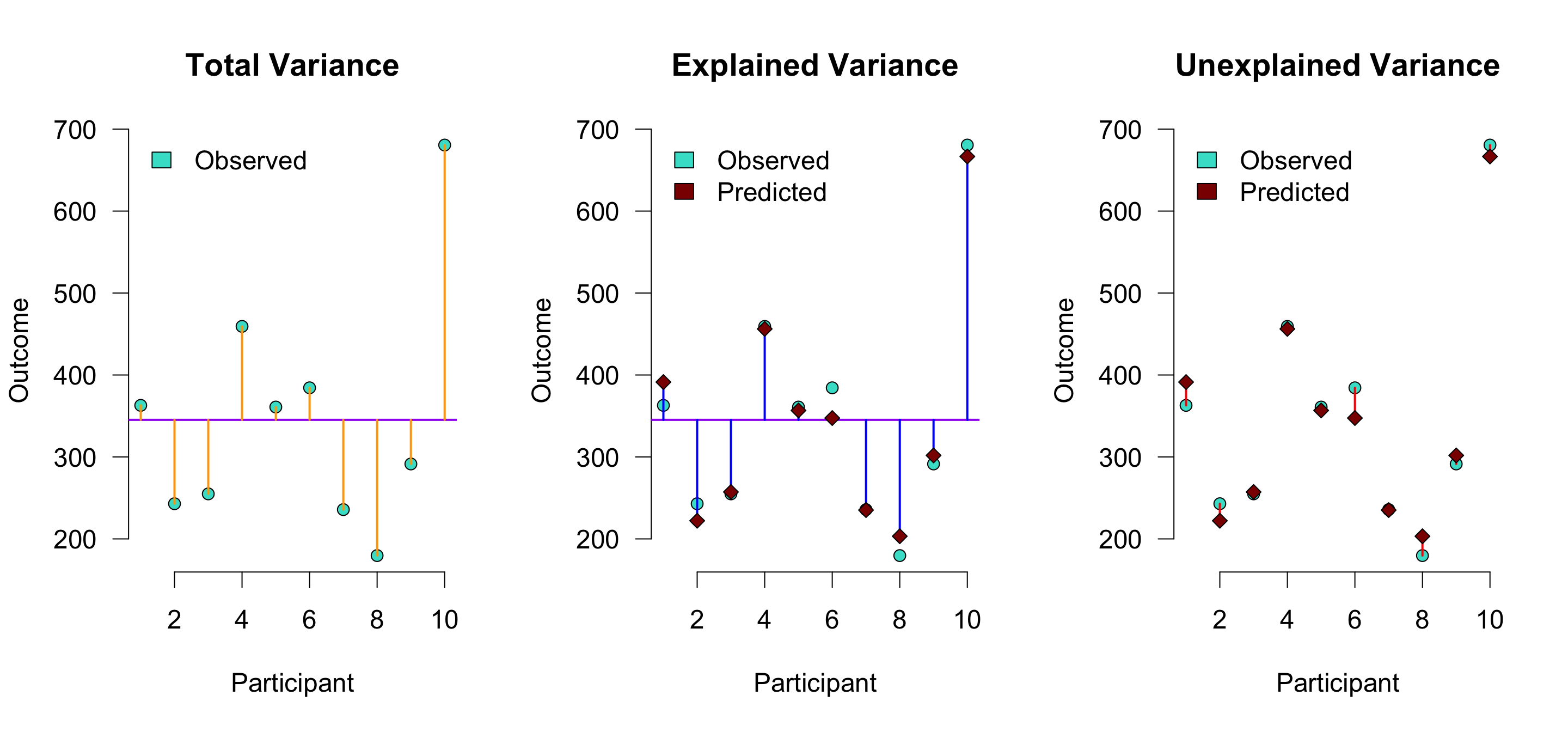
\(r^2\) is the proportion of blue to orange, while \(1 - r^2\) is the proportion of red to orange

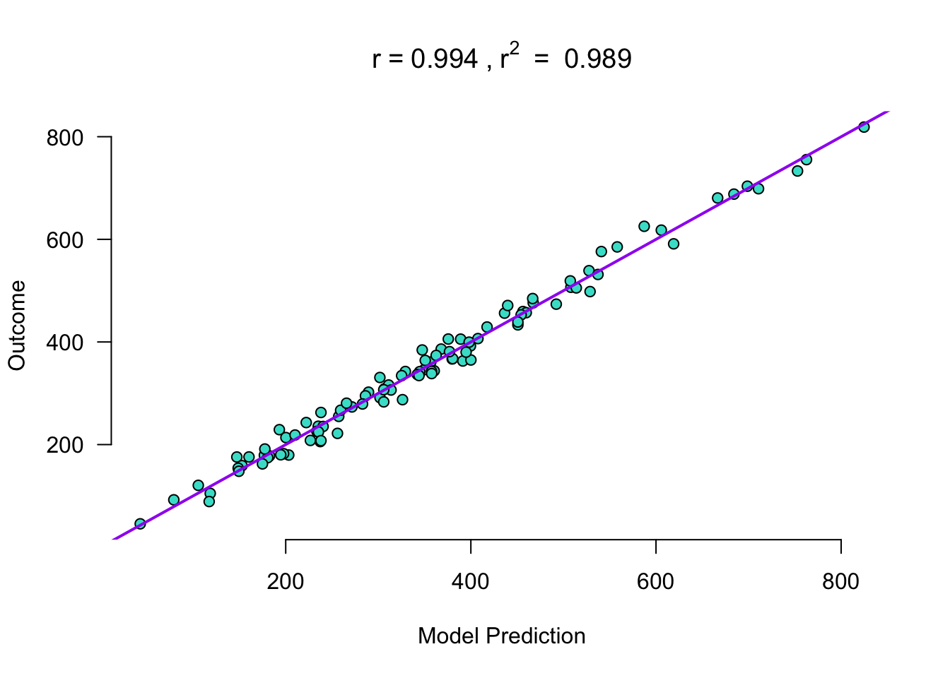
Expected vs. observed

Turn quantitative into ordinal?!

## Round to number of cups of coffee, always rounding down
data$cups.coffee <- data$ml.coffee %/% 150

Interaction in hierarchical regression

Does the interaction add anything?

Model	R²	Adjusted R²	R² change	F change	df1	df2	p
M₀	0.000	0.000	0.000		0	99
M₁	0.912	0.910	0.912	504.412	2	97	< .001
M₂	0.989	0.988	0.076	643.753	1	96	< .001

Note. M₁ includes hours.awake, ml.coffee
Note. M₂ includes hours.awake, ml.coffee, hours.awake:ml.coffee

Centering

With an interaction, \(b_1\) and \(b_2\) are effects when the other predictor is 0
Grand mean centering subtracts the mean from every score, so 0 now means average
Leaves \(b_3\) alone, but changes interpretation of \(b_1\) and \(b_2\)

	Not centered	Centered
\(b_1\) (hours.awake)	-3.612, at 0 ml coffee	23.013, at the mean (260 ml)
\(b_2\) (ml.coffee)	0.266, at 0 hours awake	1.269, at the mean (9.8 hours)
\(b_3\) (interaction)	0.102	0.102

Impact of centering grows as the interaction effect grows

Process module or linear regression?

	Linear regression	Process module
\(b_3\) (interaction)	0.102	0.102
\(b_1\), \(b_2\)	-3.612, 0.266 (not centered)	23.013, 1.269 (centered by default)
Test	\(t\)	\(z\), SEs slightly smaller (\(\times\) 0.98 here)
Also gives	\(R^2\) change, assumption checks	Simple slopes

Same estimates after unticking Mean-centered moderation in Process

JASP

Closing

Recap

Interactions still matter with continuous predictors
Continuous interactions can be assessed with:
- Linear regression
- Process module

Exam note

Keep the default settings of each analysis, no need to center by hand
- Process module centers for you (Mean-centered moderation)
- Linear regression does not center
So \(b_1\) and \(b_2\) differ between the two analyses
- Process gives the effect at the mean of the other predictor
- Linear regression gives the effect when the other predictor is 0
The interaction \(b_3\) is the same in both
Check the assumptions in Linear Regression, not in the Process module
- VIF in the model without the interaction
- Checking the assumptions (lecture 21)

Next Time

Association between categorical variables: chi-squared test (lecture 28)

Recommended Exercises

Contact