28. Chi-squared test

Contingency Tables

Johnny van Doorn

University of Amsterdam

11 November 2026

In this lecture we aim to:

Discuss association between categorical variables
- Contingency tables
Show this test in JASP

Reading: Chapter 16 (§16.1–16.10)

\(\chi^2\) test

Relation between categorical variables

\(\chi^2\) test

A “chi-squared test”, also written as \(\chi^2\) test, is any statistical hypothesis test wherein the sampling distribution of the test statistic is a chi-squared distribution when the null hypothesis is true. Without other qualification, ‘chi-squared test’ often is used as short for Pearson’s chi-squared test.

Chi-squared tests are often constructed from a Lack-of-fit sum of squared errors. A chi-squared test can be used to attempt rejection of the null hypothesis that the data are independent.

Source: wikipedia

\(\chi^2\) test statistic

\(\chi^2 = \sum \frac{(\text{observed}_{ij} - \text{prediction}_{ij})^2}{\text{prediction}_{ij}}\)

Contingency table

\(\text{observed}_{ij} = \begin{pmatrix} o_{11} & o_{12} & \cdots & o_{1j} \\ o_{21} & o_{22} & \cdots & o_{2j} \\ \vdots & \vdots & \ddots & \vdots \\ o_{i1} & o_{i2} & \cdots & o_{ij} \end{pmatrix}\)

\(\text{prediction}_{ij} = \begin{pmatrix} p_{11} & p_{12} & \cdots & p_{1j} \\ p_{21} & p_{22} & \cdots & p_{2j} \\ \vdots & \vdots & \ddots & \vdots \\ p_{i1} & p_{i2} & \cdots & p_{ij} \end{pmatrix}\)

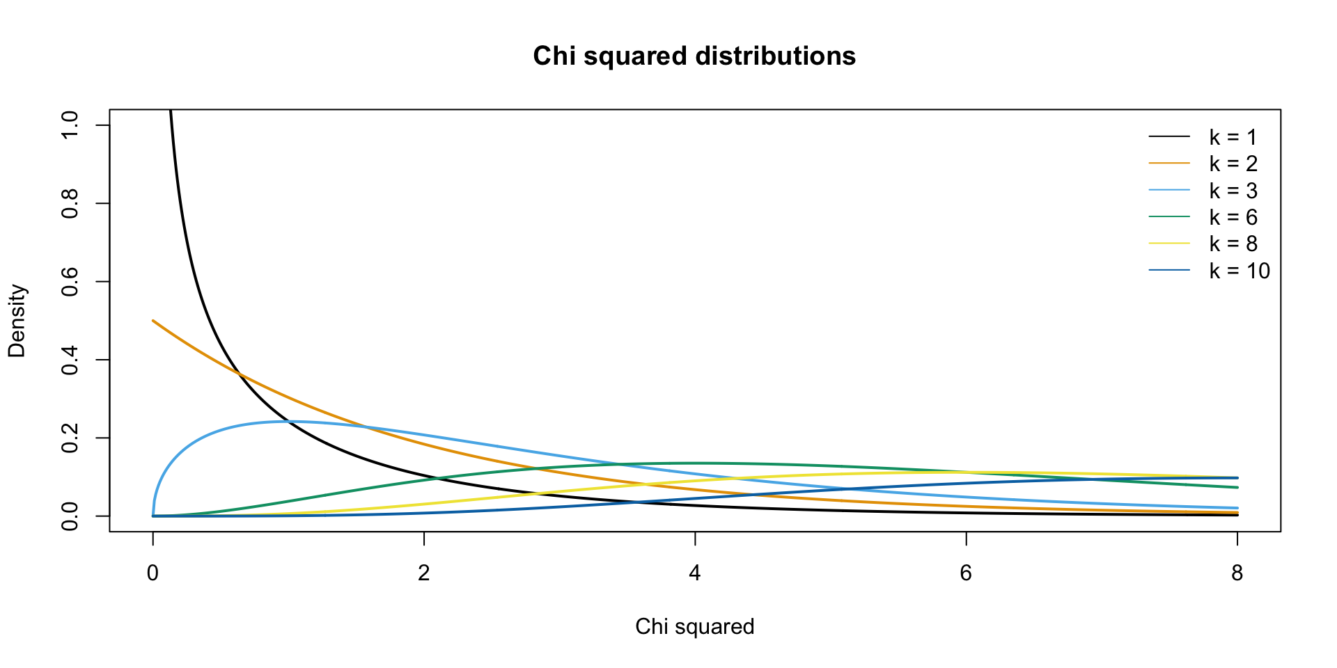
\(\chi^2\) distribution

The \(\chi^2\) distribution describes the test statistic under the assumption of \(H_0\), given the degrees of freedom.

\(df = (r - 1) (c - 1)\) where \(r\) is the number of rows and \(c\) the number of columns.

Assumptions

Independence
- Each person contributes to one cell only (no repeated measures)
Expected frequencies not too small
No normality assumption (categorical variables are not continuous)

Experiment

Data

Calculating \(\chi^2\)

observed <- table(results[, c("Lecture", "Personality")])
observed

         Personality
Lecture   Extrovert Introvert
  Digital        13        10
  Live           15        26

\(\text{observed}_{ij} = \begin{pmatrix} 13 & 10 \\ 15 & 26 \\ \end{pmatrix}\)

Calculating the model predictions

\(\text{prediction}_{ij} = \text{expected}_{ij} = \frac{\text{row total}_i \times \text{column total}_j}{n }\)

n   <- sum(observed)
totExt <- colSums(observed)[1]
totInt  <- colSums(observed)[2]
totDig  <- rowSums(observed)[1]
totLiv <- rowSums(observed)[2]

addmargins(observed)

         Personality
Lecture   Extrovert Introvert Sum
  Digital        13        10  23
  Live           15        26  41
  Sum            28        36  64

Prediction under \(H_0\) for one cell

Under \(H_0\), lecture type and personality are independent
- \(P(A \text{ and } B) = P(A) \times P(B) \qquad P(A \mid B) = P(A)\)
So the share of extroverts is the same for digital and live

pDigital   <- totDig / n    # P(digital), row total / n
pExtrovert <- totExt / n    # P(extrovert), column total / n
pDigital * pExtrovert * n   # predicted number of digital extroverts

Digital 
10.0625

\(\small \text{prediction}_{\text{digital, extrovert}} = \underbrace{\dfrac{23}{64}}_{P(\text{digital})} \times \underbrace{\dfrac{28}{64}}_{P(\text{extrovert})} \times \underbrace{\;64\;}_{n} = \dfrac{\text{row total} \times \text{column total}}{n} = 10.06\)

Calculating the model

\(\text{prediction}_{ij} = \text{expected}_{ij} = \frac{\text{row total}_i \times \text{column total}_j}{n }\)

         Personality
Lecture   Extrovert Introvert
  Digital   10.0625   12.9375
  Live      17.9375   23.0625

\(\text{prediction}_{ij} = \begin{pmatrix} 10.0625 & 12.9375 \\ 17.9375 & 23.0625 \\ \end{pmatrix}\)

Error = Observed - Model

observed

         Personality
Lecture   Extrovert Introvert
  Digital        13        10
  Live           15        26

modelPredictions

         Personality
Lecture   Extrovert Introvert
  Digital   10.0625   12.9375
  Live      17.9375   23.0625

observed - modelPredictions

         Personality
Lecture   Extrovert Introvert
  Digital    2.9375   -2.9375
  Live      -2.9375    2.9375

Calculating \(\chi^2\)

\(\chi^2 = \sum \frac{(\text{observed}_{ij} - \text{prediction}_{ij})^2}{\text{prediction}_{ij}}\)

# Calculate chi squared
chi.squared <- sum((observed - modelPredictions)^2 / modelPredictions)
chi.squared

[1] 2.379707

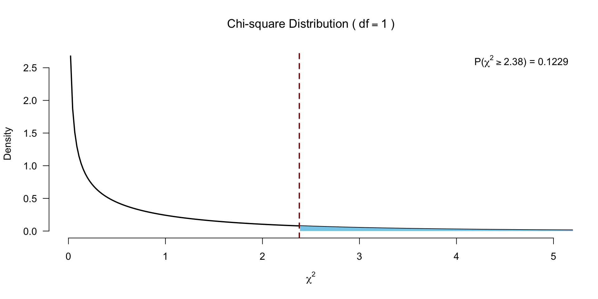
Testing for significance

\(df = (r - 1) (c - 1)\)

\(P\)-value

Checking expected counts

With 2 \(\times\) 2 tables, no expected values should be below 5
In larger tables, all expected counts should be greater than 1 and no more than 20% less than 5

modelPredictions

         Personality
Lecture   Extrovert Introvert
  Digital   10.0625   12.9375
  Live      17.9375   23.0625

Smallest expected count is 10.06, so Pearson’s \(\chi^2\) holds
In JASP via Cells → Counts → Expected

Fisher’s exact test

Calculates the exact probability of the \(\chi^2\) statistic for small samples (at least one cell of the table has an expected count smaller than 5), when the \(\chi^2\) approximation does not yet suffice.

Calculate all possible permutations.

Expected cell size < 5

Standardized residuals

\(\text{standardized residuals} = \frac{ \text{observed}_{ij} - \text{prediction}_{ij} }{ \sqrt{ \text{prediction}_{ij} } }\)

(observed - modelPredictions) / sqrt(modelPredictions)

         Personality
Lecture    Extrovert  Introvert
  Digital  0.9260297 -0.8166815
  Live    -0.6935806  0.6116806

Effect size

Odds ratio based on the observed values

observed

         Personality
Lecture   Extrovert Introvert
  Digital        13        10
  Live           15        26

Odds visualized

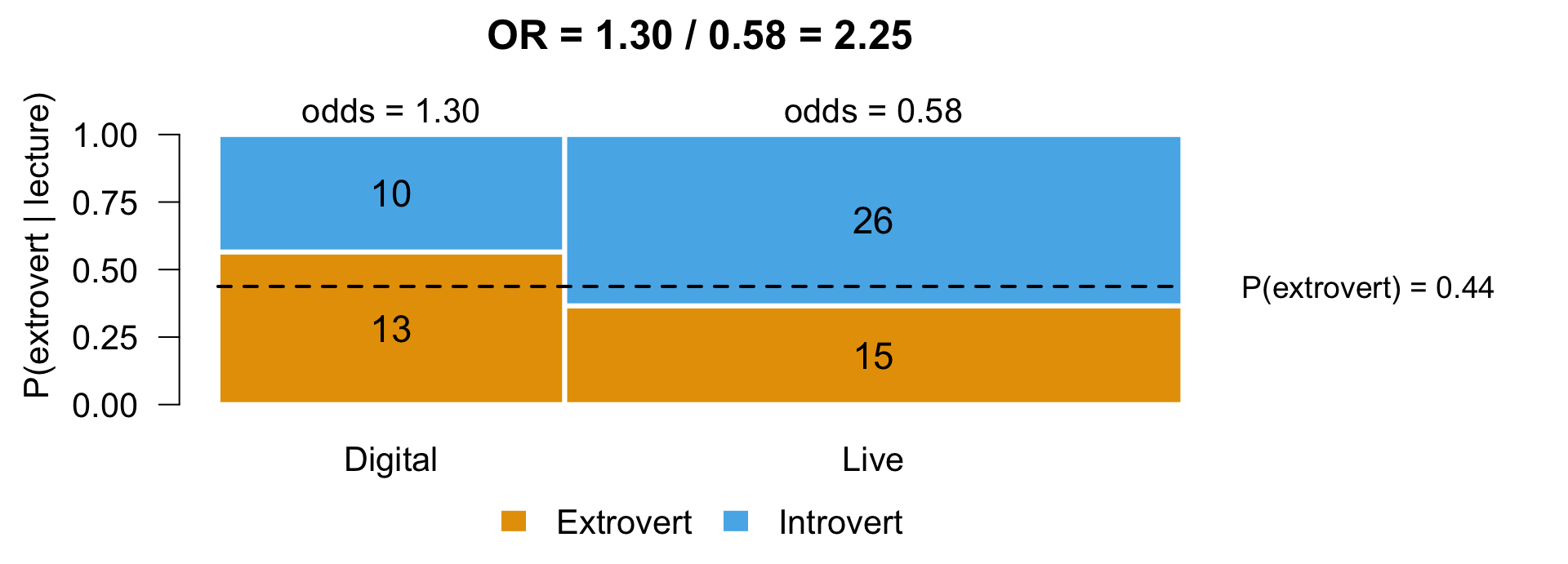
Bar height is \(P(\text{extrovert} \mid \text{lecture})\), bar width the group size
\(\text{odds}_{\text{digital}} = \dfrac{P(\text{extrovert} \mid \text{digital})}{P(\text{introvert} \mid \text{digital})} = \dfrac{13 / 23}{10 / 23} = \dfrac{13}{10}\)
Under \(H_0\) both bars split at the dashed line, \(P(\text{extrovert})\), so \(OR = 1\)

Odds

         Personality
Lecture   Extrovert Introvert
  Digital        13        10
  Live           15        26

The extrovert/introvert ratio for digital and live audiences:

\(\text{odds}_{\text{digital}} = \frac{\text{extrovert}}{\text{introvert}} = \frac{ 13 }{ 10 } = 1.30\)
\(\text{odds}_{\text{live}} = \frac{\text{extrovert}}{\text{introvert}} = \frac{ 15 }{ 26 } = 0.58\)

In the digital responses, there are +- 1.30 times as many extroverts as introverts. In the live responses, there are +- 0.58 times as many extroverts as introverts.

Odds ratio

Is the ratio of these odds.

\(OR = \dfrac{\text{odds}_{\text{digital}}}{\text{odds}_{\text{live}}} = \dfrac{13 / 10}{15 / 26} = \dfrac{1.30}{0.58} = 2.25\)

\(OR = 1\) means the same odds in both groups (no association)

Odds, the other way around

         Personality
Lecture   Extrovert Introvert
  Digital        13        10
  Live           15        26

Alternatively, we can look at the ratios of digital/live for extroverts and introverts:

\(\text{odds}_{\text{extrovert}} = \frac{\text{digital}}{\text{live}} = \frac{ 13 }{ 15 } = 0.87\)
\(\text{odds}_{\text{introvert}} = \frac{\text{digital}}{\text{live}} = \frac{ 10 }{ 26 } = 0.38\)

For the extroverts, there are +- 0.87 times as many digital viewers as live viewers. For the introverts, there are +- 0.38 times as many digital viewers as live viewers.

Odds ratio, the other way around

\(OR = \dfrac{\text{odds}_{\text{extrovert}}}{\text{odds}_{\text{introvert}}} = \dfrac{13 / 15}{10 / 26} = \dfrac{0.87}{0.38} = 2.25\)

\(\dfrac{\text{odds}_{\text{digital}}}{\text{odds}_{\text{live}}} = \dfrac{\text{odds}_{\text{extrovert}}}{\text{odds}_{\text{introvert}}} = 2.25\)

Same OR, whichever way you read the table

For these data, the odds of watching digitally were approximately 2.25 times higher for extroverts than for introverts. The odds ratio also accounts for the scores in both conditions—watching digitally and watching live—by comparing the odds of watching digitally to live viewing across both personality types.

Odds ratio shortcut

\(\begin{pmatrix} a & b \\ c & d \\ \end{pmatrix} = \begin{pmatrix} 13 & 10 \\ 15 & 26 \\ \end{pmatrix}\)

\(OR = \dfrac{a / b}{c / d} = \dfrac{a / c}{b / d} = \dfrac{a \times d}{b \times c} = \dfrac{13 \times 26}{10 \times 15} = 2.25\)

JASP shows the log odds ratio by default, where \(\log(OR) = 0\) means no association

More examples

Book example

200 cats trained to dance, with food or affection as reward
Training (food or affection, not both)
Dance (the cat learned to dance or it did not)

cats <- matrix(c(28, 48, 10, 114), nrow = 2,
               dimnames = list(Training = c("Food", "Affection"),
                               Dance    = c("Yes", "No")))
addmargins(cats)

           Dance
Training    Yes  No Sum
  Food       28  10  38
  Affection  48 114 162
  Sum        76 124 200

\(\chi^2\) and \(p\)-value

# row total x column total / n, for every cell
catsModel <- outer(rowSums(cats), colSums(cats)) / sum(cats)
catsChi   <- sum((cats - catsModel)^2 / catsModel)
catsChi

[1] 25.35569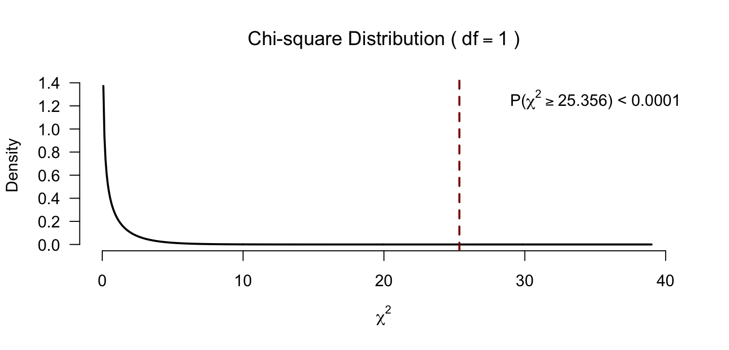

Odds visualized

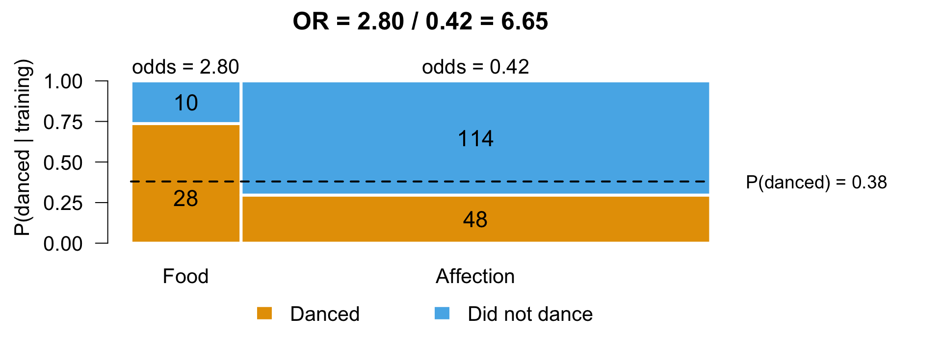
Bar height is \(P(\text{danced} \mid \text{training})\), bar width the group size
\(\text{odds}_{\text{food}} = \dfrac{P(\text{danced} \mid \text{food})}{P(\text{did not dance} \mid \text{food})} = \dfrac{28 / 38}{10 / 38} = \dfrac{28}{10}\)
Under \(H_0\) both bars split at the dashed line, \(P(\text{danced})\), so \(OR = 1\)

Independent predictors

Accidents in the driving simulator from lecture 17 (alcohol \(\times\) speed)

Alcohol / speed	none	some	much
none	20	20	20
some	20	20	20
much	20	20	20

\(\text{prediction}_{ij} = \frac{60 \times 60}{180} = 20\) in every cell, same as observed
Balanced design, so \(\chi^2(4) = 0.00\) (\(p = 1.00\)) and alcohol and speed are independent

JASP

Closing

Recap

Chi-square test assesses categorical associations
Can be used to assess (in)dependence between predictors
Has test statistic (χ²) + effect size (odds ratio)

Next Time

Bayesian ANOVA (lecture 29)

Recommended Exercises

Labcoat Leni 16.1

Daniels (2012): The impact of sexualized images on women’s self-evaluations

Is the type of image viewed related to self-objectification?

picture: performance vs. sexualized athlete images
theme_present: self-objectification theme present or absent
self_evaluation: counts

Data (.jasp) · Results (.jasp) · Results (.html)

Labcoat Leni 16.2

Beckham (1929): Is the Black American happy?

Do yes/no answers differ between professions? One test for each of the three questions.

profession: the respondent’s job
response: yes or no
happy, you_happy, should_be_happy: counts for each question

Data (.jasp) · Results (.jasp) · Results (.html)

Note

This study asked three simple questions, yet the data are fascinating. Pioneering school psychologist Albert Sidney Beckham (1897–1964) raised further hypotheses that could be tested, it unearthed very different views in different professions, and it illuminated very important social and psychological issues.

Contact