3. Statistical Reasoning

NHST and sampling distributions

Author

Affiliation

Johnny van Doorn

University of Amsterdam

Published

4 September 2026

In block 1 we aim to:

Discuss NHST concepts
Introduce JASP
Correlation
Linear model (regression)

Reading: Chapters 1–8.8

In this lecture we aim to:

Introduce the S in SSR
- The book, the course, and how to study for it
Repeat some stats concepts from RMS
- “Logic” behind common hypothesis testing
- Four scenario’s in statistical decision making
Sampling distributions
- The binomial distribution

Reading: Chapters 1, 2, 3 (§1.1–1.8, §2.1–2.9, §3.1–3.8)

Statistics in SSR

The stats half of SSR

Two halves running side by side: reasoning (arguments, rationality, critical thinking) and statistics. These are the statistics lectures.

Block 1: getting back into statistics
- NHST, correlation, regression
Block 2: comparing means
- t-tests, ANOVA, chi-square, non-parametric tests
Block 3: multiple predictors
- multiple regression, mediation, moderation

Each block closes with an interim exam.

What will you learn?

Not just computing the right number. Three levels, and we want all three:

Statistical literacy: knowing the concepts and working the tools
- Identify, describe, translate, interpret, read, compute
Statistical reasoning: understanding why and how a method works
Statistical thinking: using it in the wild
- Apply: what method fits this situation?
- Critique: reflect on the work of others
- Evaluate: assign value to that work
- Generalize: what does variation mean in the large scheme of life?

Source: ARTIST

Book

Field, Discovering Statistics Using JASP.

Block 1: Chapters 1 through 8.8 (skipping Chapter 6)
Companion website: discoverjasp.com
You have the book, glossary included, during the exam

Sections A to D

Every section carries a letter for difficulty, each rhyming with what it does to your brain:

A is for brain Attain: everyone should get something out of these
B is for brain Bane: more knowledge needed, at times a source of unhappiness
C is for brain Complain: final-year or master’s material
D is for brain Drain: difficult enough to drain Field’s own brain

In this course we focus mostly on A and B.

Characters

Worth looking out for:

Cramming Sam: key points of a chapter, summarized
Smart Alex: end-of-chapter tasks, answers on the website
Labcoat Leni: real data from real studies
Oliver Twisted: extra material on the website
Jane Superbrain: advanced tangents

Software

JASP
- Download the latest version (0.98.1) from the website
- Your main tool in SSR for handling data and conducting analyses
- Also available in the virtual UvA desktop and at any UvA computer
R
- Statistical programming language, under the hood of JASP and my SSR slides
- Very optional, sometimes included in the slide for those interested
- R (language pack) and Rstudio (coding environment) available on the exam computers

Study tips

Read the chapter before the lecture. The lecture is then your second pass, not your first
Practice statistics in JASP yourself: WA, Smart Alex tasks, and Labcoat Leni examples
For a deeper dive, play with the applets, consult the JASP Video Library, ask questions on the Discussion Board or have a chat with Roenny

Exam

Statistics proportional to lectures (IE1: 40%, IE2: 60%, IE3: 50%)
MC, OEQ, Fill-in-the-blank
You have JASP and the book, glossary included, during the exam
See the trial exam in Ans during the exam week

Null Hypothesis
Significance Testing

Measurement Tool

Suppose we want to find out whether someone is a physics expert.

A multiple-choice test, true/false
- Q1: The vacuum state in quantum field theory is not actually empty but contains fluctuations of virtual particles.
10 items in total
When do we decide someone is an expert?

Empirical Cycle

Observation Someone seems to be very knowledgeable on physics
Induction They could be an expert in the field
Deduction $H_0$: P: $\theta = 0.5$ → C: They were guessing
Deduction $H_A$: P: $\theta > 0.5$ → C: They have knowledge
Deduction $H_A$: P: data $\neq$ EV → C: The candidate is expert
Testing Choose $\alpha$ and Power
Evaluation Make a decision

Two hypotheses

$H_0$

Skeptical point of view
No effect
No preference
No correlation
No difference

$H_A$

Refute Skepticism
Effect
Preference
Correlation
Difference

What if they were just guessing?

What happens if they are guessing?

Binomial distribution

\[P(k \text{ success out of } n \text{ trials} \mid \text{probability } p) = {n\choose k}p^k(1-p)^{n-k}\] where \[ {n\choose k} = \frac{n!}{k!(n-k)!} \]

With values:

n <- 10   # Sample size
k <- 0:10 # Discrete probability space (numbers 0, 1, ..., 9, 10)
p <- .5   # Probability of correct guess

The null distribution

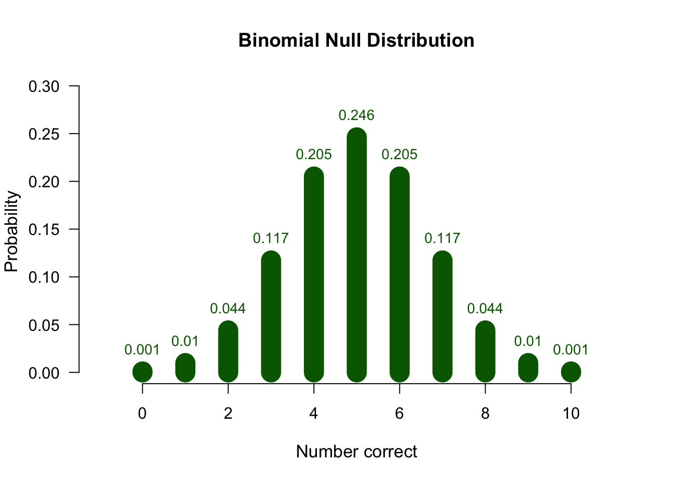
What we just did has a name

The number of correct answers is a test statistic.

A statistic that summarizes the data and is used for hypothesis testing, because we know how it’s distributed under different hypotheses

Common test statistics:

Number of heads
Sum of dice
$t$-statistic
$F$-statistic
$\chi^2$-statistic
etc…

What do those bar heights mean?

Objective Probability
Relative frequency in the long run

How surprising is the data?

Testing

The candidate had 8 items correct. Can we conclude they are a physics expert?

As you can see from the distribution of novice scores, we cannot conclude that by definition.
What we can do is indicate how rare 8 is in a novice.

Formulating the hypotheses

If they are guessing ($H_0$), the expected value (EV) is 5 correct answers out of 10

$H_0: EV = 5$

If they are an expert, the EV is greater than 5 correct answers out of 10

$H_A: EV > 5$

We could also formulate our $H_0$ and $H_A$ more abstract:

$H_0:$ the candidate is novice

$H_A:$ the candidate is expert

Making the decision

Due to getting ``lucky’’, a novice can also score greater than 5, but how strict should we be in our decision that someone is an expert?

$\alpha$$ determines how strict we are in our decision to reject the null hypothesis (historically set to 5%).

Candidate scored 8 items correct. If they would have been guessing, the probability to score 8 correct or more, is greater than 5%.

Therefore, for $\alpha = 0.05$ we conclude that our candidate is a novice, based on this trial.

P-value

Conditional probability of the observed test statistic or more extreme assuming the null hypothesis is true.

Reject $H_0$ when:

$p$-value $\leq$ $\alpha$

P-value in $H_{0}$ distribution

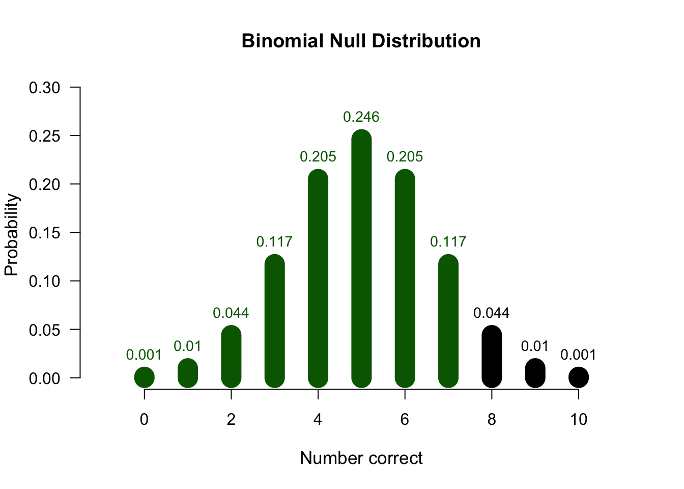
\[P(k \geq 8 \mid H_0) = 0.044 + 0.01 + 0.001 = 0.055\]

P-value and $\alpha$

Alpha determines how willingly we reject the null hypothesis:

Increase $\alpha$ = reject null hypothesis more often
- Increases Type I error rate
- Decreases Type II error rate
Historically set to 0.05, but widely criticized (see Jane Superbrain 3.1)

No scientific worker has a fixed level of significance at which from year to year, and in all circumstances, he rejects hypotheses; he rather gives his mind to each particular case in the light of his evidence and his ideas. (Fisher, 1956)

$\alpha$ dictates the rejection region

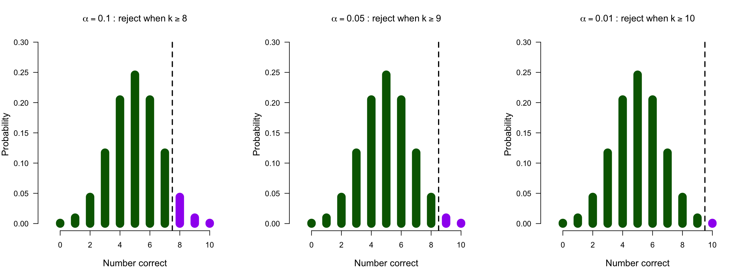
The stricter the $\alpha$, the further into the tail the region starts. Our candidate’s 8 would only count as “significant” at $\alpha = .10$.

Misconceptions about the p-value

A significant result means that the effect is important
- Significance = effect size + sample size
A non-significant result means that the null hypothesis is true
A significant result means that the null hypothesis is false

What can go wrong?

Neyman-Pearson Paradigm

Neyman

Pearson

Fisher asked how surprising is this data? Neyman and Pearson asked a different question: which mistakes am I willing to make, and how often?

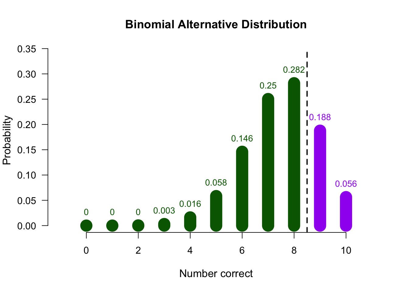
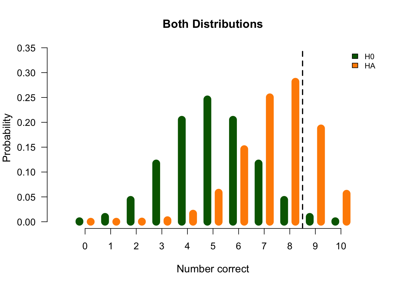
Alternative Distribution

But we have no clue what this distribution could look like.

For now let’s assume the probability of answering an item correctly is .75

Both distributions at once

Decision table

The two ways to be wrong: $\alpha$ and $\beta$

$\alpha$ — Type I error

Incorrectly reject $H_0$
False positive
Threshold for “significance”
Criteria often 5% but heavily criticized

$\beta$ — Type II error

Incorrectly accept $H_0$
False negative
Criteria often 20%
Distribution depends on sample size

The two ways to be right: power and $1-\alpha$

Power — correctly reject $H_0$

True positive
Power $= 1 - \beta$
Criteria often 80%
Depends on sample size

$1-\alpha$ — correctly accept $H_0$

True negative

Applet

Play around with this app to get an idea of the probabilities

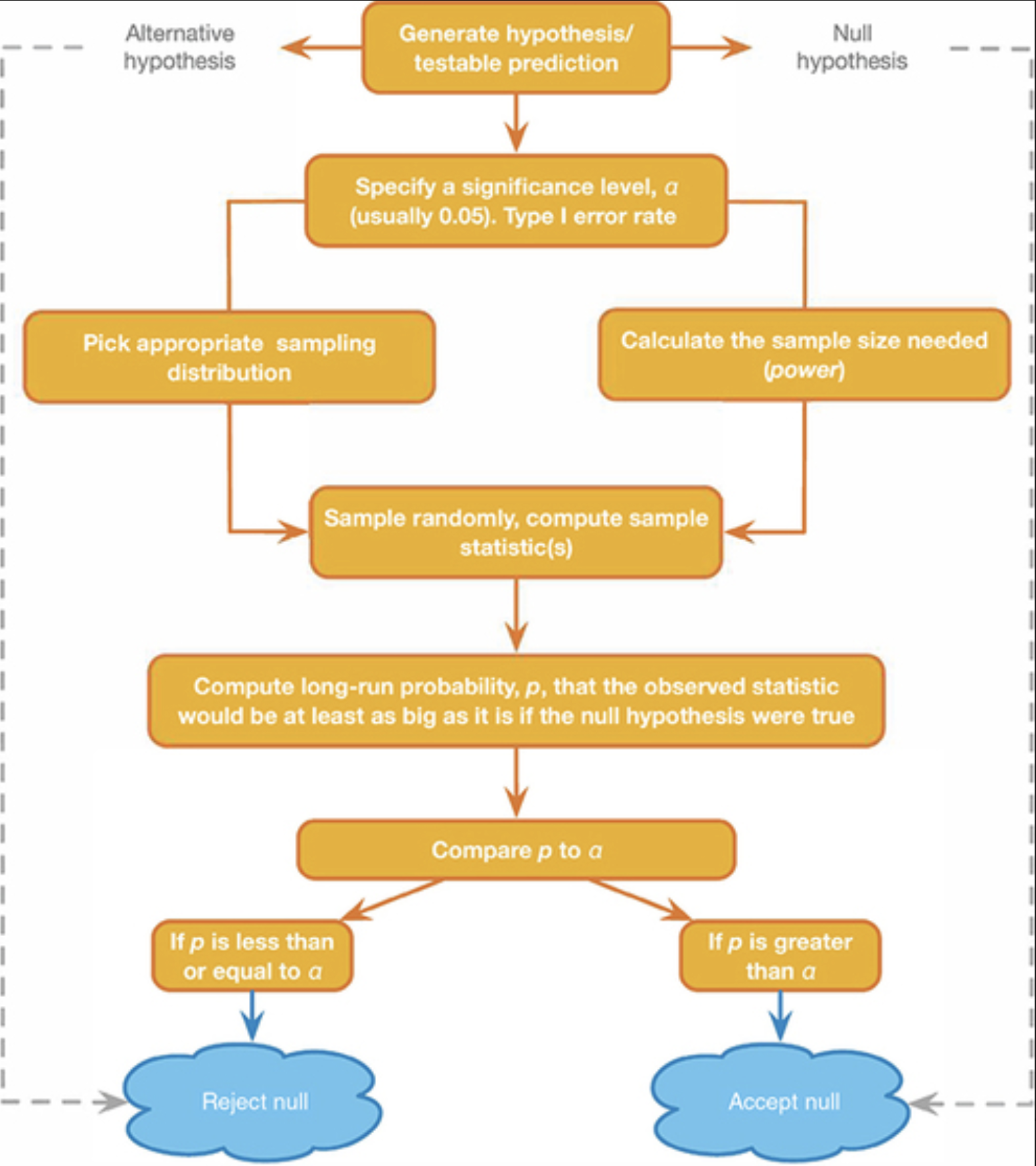
NHST Reasoning Scheme

Closing

Next Time

JASP
- Descriptive statistics
- Data visualizations
Describing and visualizing data

Bored?

Contact