9. Linear Model (Regression)
One predictor
In this lecture we discuss:
- Linear model
- Theory
- Assumptions
- In JASP
- Predictions and model fit
Reading: Chapter 8 (§8.1–8.8)
Last week
Last week: correlation & NHST
- \(COV_{xy}\): association between two variables, in the original measurement units
- \(r\): completely standardized: \(r_{xy} = \frac{COV_{xy}}{s_x s_y}\)
- Get \(p\) by converting to \(t\): \(t_r = \frac{r \sqrt{N-2}}{\sqrt{1 - r^2}}\)
- Partial correlation: the same association, holding a third variable constant
Note on one-sided vs. two-sided testing
A choice in the analysis before seeing the data (i.e., informed by the research question, not the result).
- Two-sided
- Safer choice if unsure about the direction
- “Spending \(\alpha\)” on two tails needs a more extreme test statistic to reach significance
- One-sided
- Blind to an effect in the opposite direction
- Same \(\alpha\), but the \(\alpha \%\) rejection area is in 1 tail
- Higher power, relevant when \(N\) is small (expensive studies, rare cases)
The data
Predict album sales (x 1,000 copies) based on the advertising budget (x £1,000).
The data
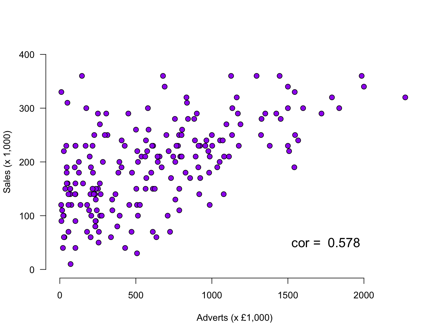
Two different units
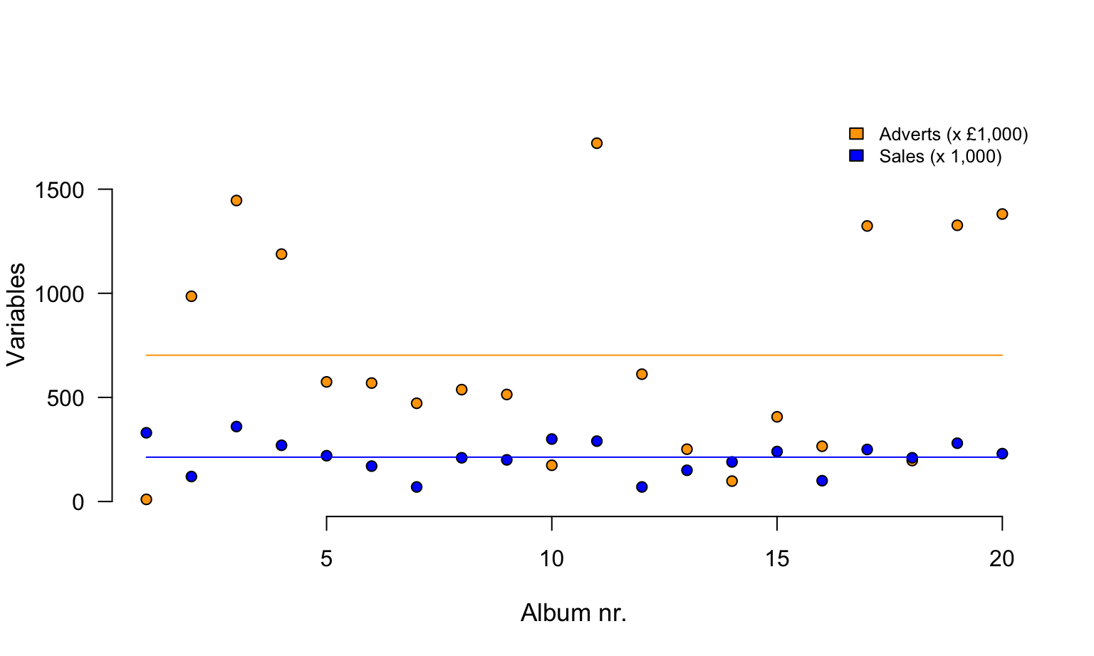
A deviation of 100 means something different in each variable
Standardize
\[z_i = \frac{x_i - \bar{x}}{sd_x}\]
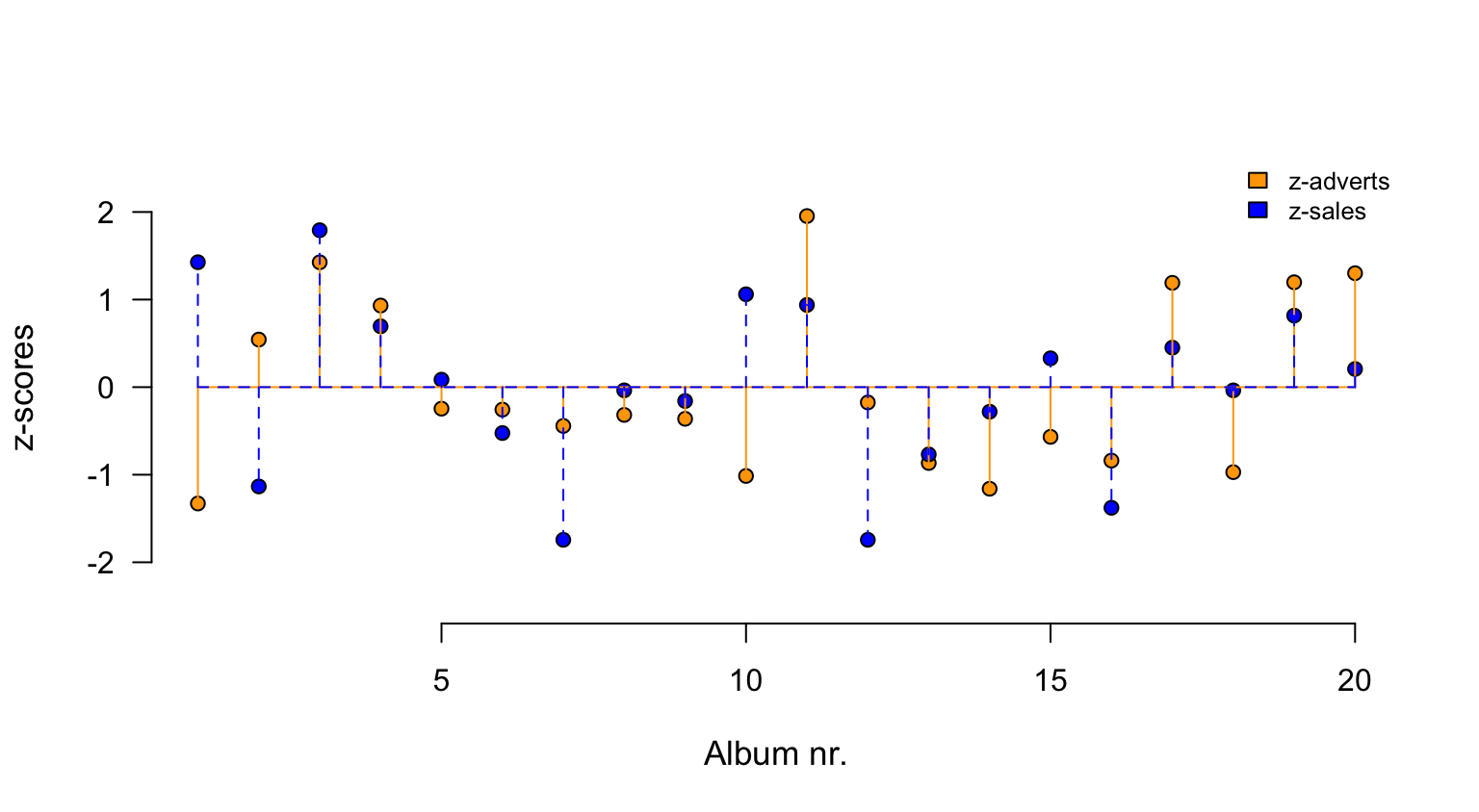
Mean = 0 and sd = 1, now the deviations are comparable.
Correlation is the covariance of z-scores
\[z_i = \frac{x_i - \bar{x}}{s_x} \qquad\qquad r_{xy} = \frac{COV_{xy}}{s_x s_y} = COV_{z_x z_y}\]
z.adverts <- (adverts - mean(adverts)) / sd(adverts)
z.sales   <- (sales   - mean(sales))   / sd(sales)

cov(z.adverts, z.sales)
[1] 0.5784877cor(adverts, sales)[1] 0.5784877If we standardize both variables first, the covariance is the correlation.
Three levels of standardization
cov(adverts, sales) # original scale[1] 22672.02cov(adverts, sales) / (sd(adverts) * sd(sales)) # standardize x and y -> the correlation[1] 0.5784877cov(adverts, sales) / var(adverts) # only x -> today's slope[1] 0.09612449Standardizing makes a statistic universally interpretable, but you lose information
Today
- The regression slope \(b_1\): \(b_1 = r_{xy} \frac{s_y}{s_x}\)
- Same trick for significance: coefficient \(b\) \(\rightarrow t \rightarrow p\)
- Making predictions based on a model
- One predictor today, multiple predictors in block 3
Regression
(one predictor)
Regression
\[\LARGE{\text{outcome} = \text{model prediction} + \text{error}}\]
In statistics, linear regression is a linear approach for modeling the relationship between a scalar dependent variable y and one or more explanatory variables denoted X. The case of one explanatory variable is called simple linear regression.
\[\LARGE{Y_i = \beta_0 + \beta_1 X_i + \epsilon_i}\]
In linear regression, the relationships are modeled using linear predictor functions whose unknown model parameters are estimated from the data.
Source: wikipedia
Assumptions of the Linear Model
A selection from Field (Section 8.4.1):
- Sensitivity (Section 6.4)
- Are there outliers?
- Normality (Section 6.8)
- Are the model errors non-normally distributed?
- Linearity (Section 6.6)
- Is the association non-linear?
- Homoscedasticity (Section 6.7)
- Is there systematic model error?
The greater the assumption violation, the less reliable your results are
Sensitivity
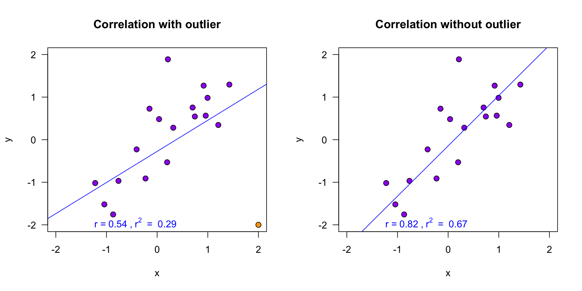
Outliers
- Extreme residuals (e.g., > 3)
- Cook’s distance (e.g., > 1)
- Check Q-Q, residuals plots, casewise diagnostics
Sensitivity
Normality
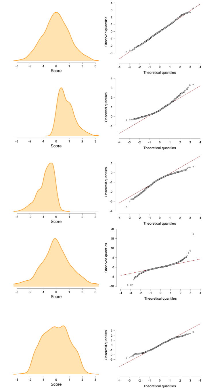
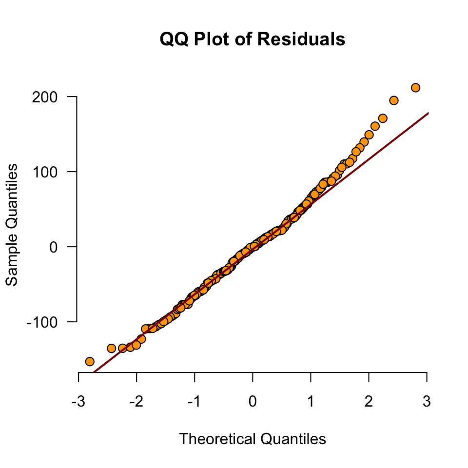
- Residuals should be normally distributed
- Look at Q-Q plot standardized residuals. Most points should be on the diagonal
- After the analysis is complete because it’s based on the residuals
- See figure 6.25
When does normality matter?
- Normality doesn’t matter in large samples (thank you CLT)
- Parameter estimation itself does not require normality
- Small samples: check the Q-Q plot of the residuals
Field, Section 6.8.3
Linearity
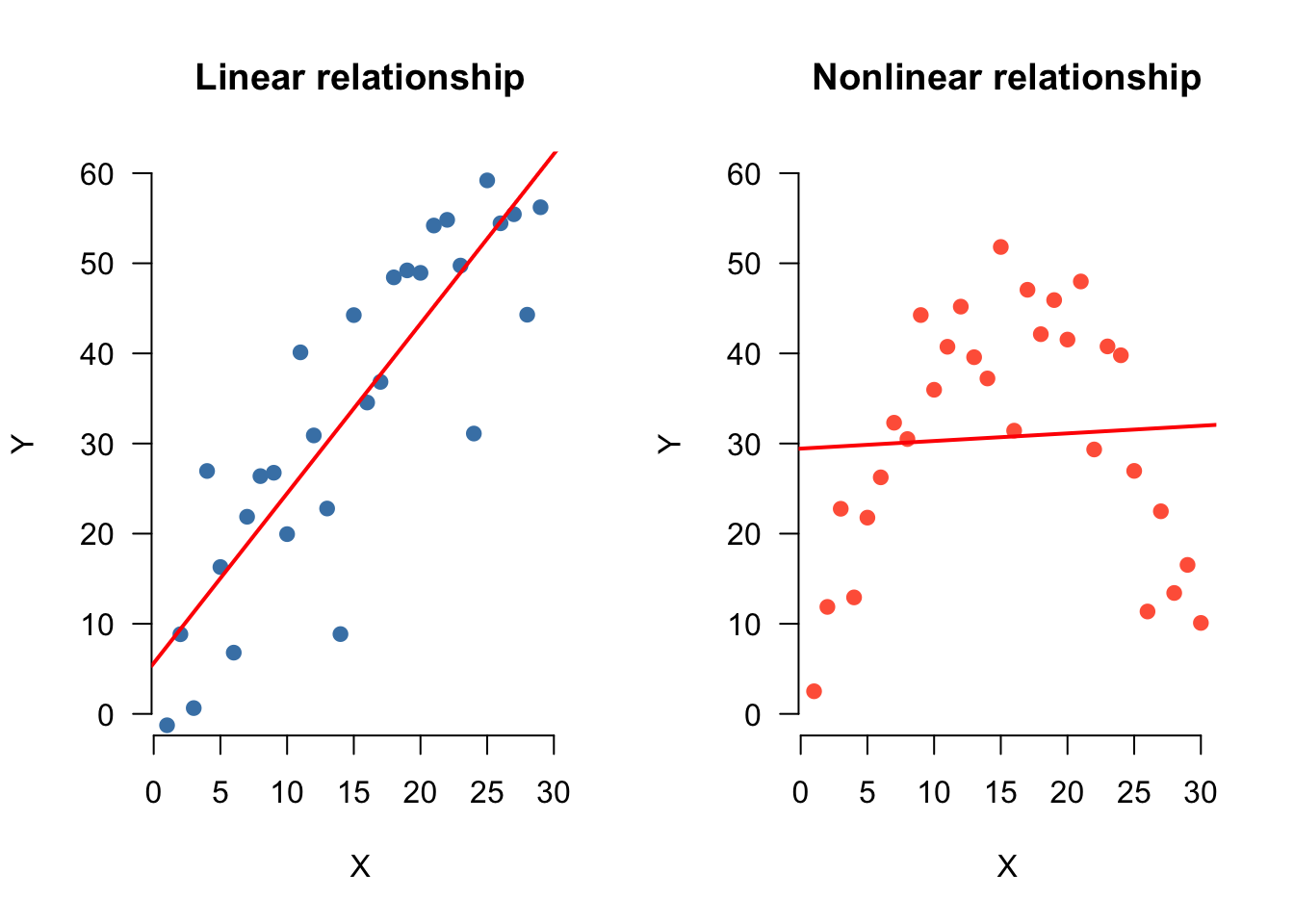
- The relationship between predictors and the outcome should be linear
- Inspect using plots:
- Scatter plots (or partial plots) of predictors vs. outcome
- Residuals vs. predicted
- See also Figure 6.28
Homoscedasticity
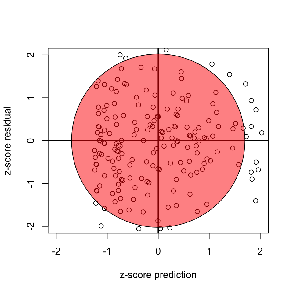
- Variance of residuals should be equal across all expected values
- Look at scatterplot of residuals vs. predicted values. Ideally it’s an uncorrelated, round cloud
- For examples of violations, see here
- After the analysis is complete because it’s based on the residuals
Calculate regression parameters
\[{sales}_i = b_0 + b_1 {adverts}_i + \epsilon_i\]
adverts  <- data$Adverts
sales    <- data$Sales
Calculate \(b_1\)
\[b_1 = r_{xy} \frac{s_y}{s_x}\]
# Calculate b1

cor.sales.adverts <- cor(sales,adverts)
sd.sales          <- sd(sales)
sd.adverts        <- sd(adverts)

b1 <- cor.sales.adverts * ( sd.sales / sd.adverts )
b1
[1] 0.09612449Calculate \(b_0\)
\[b_0 = \bar{y} - b_1 \bar{x}\]
mean.sales    <- mean(sales)
mean.adverts  <- mean(adverts)

b0 <- mean.sales - b1 * mean.adverts
b0
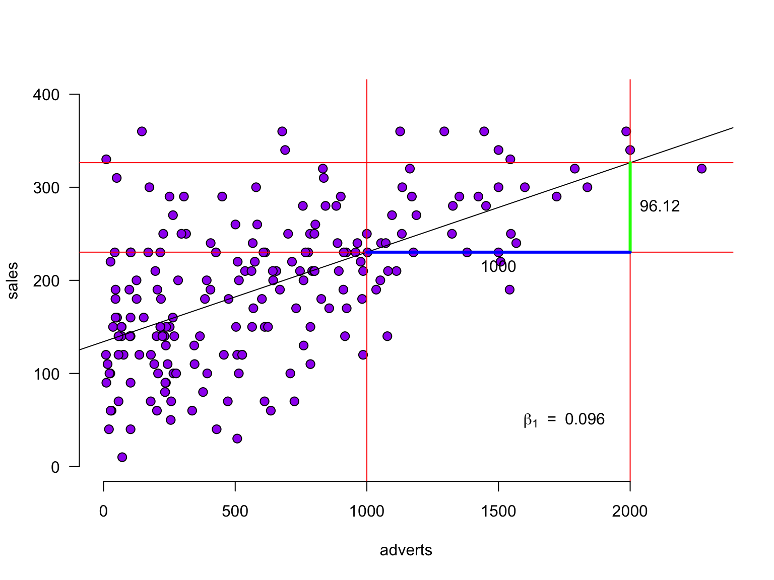
[1] 134.1399The slope
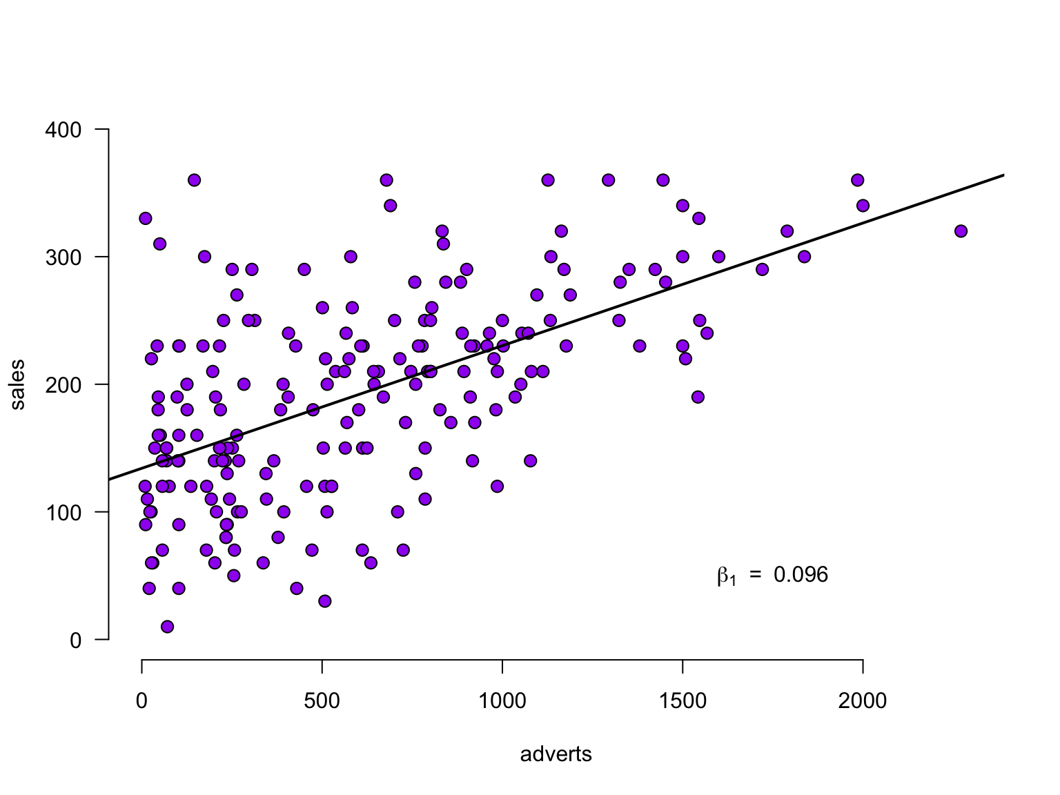
The slope
The slope - zoomed in
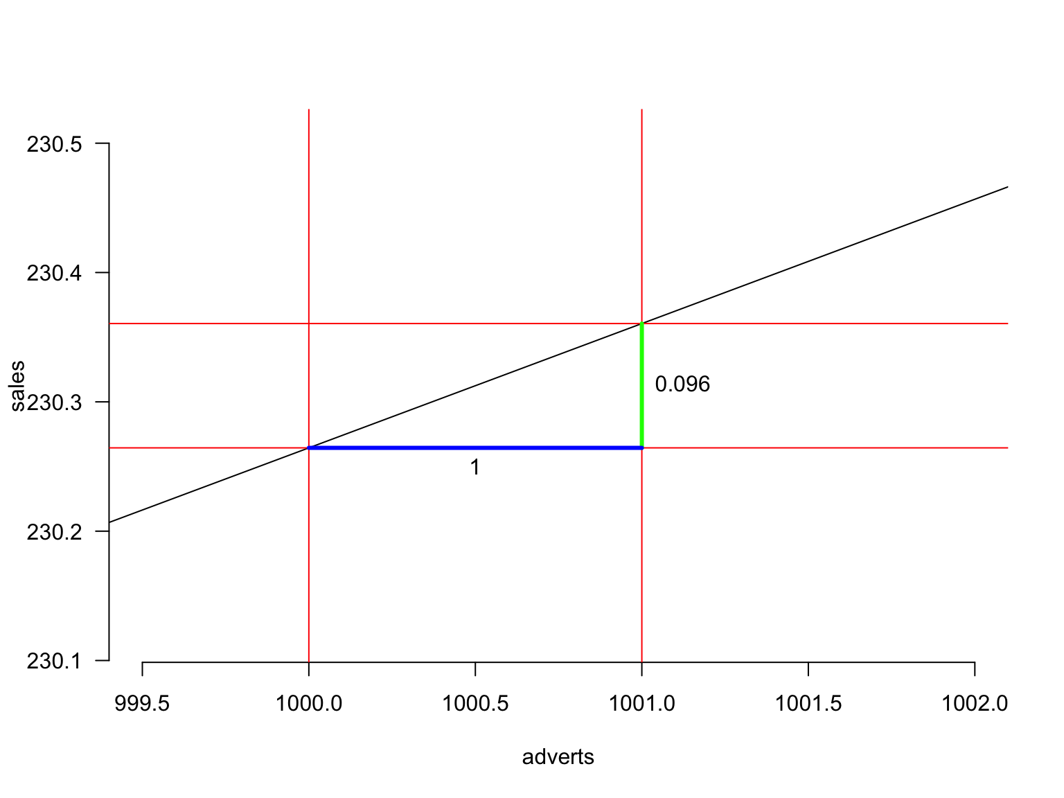
For every additional £1,000 spent on advertising, we predict sales to increase by 0.096 (x 1,000 copies)
Define regression equation
\[\widehat{sales} = {\text{model prediction}} = b_0 + b_1 {adverts}\] \[\widehat{sales} = {\text{model prediction}} = 134.14 + 0.096\times {adverts}\]
So now we can add the expected sales based on this model
prediction <- b0 + b1 * adverts
data$prediction <- round(prediction, 2)
Predicted values
Let’s have a look
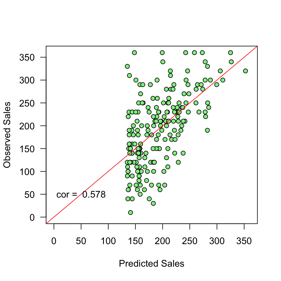
\(y\) vs \(\hat{y}\)
And lets have a look at this relation between model prediction and observed
Error
The error (residual) is the difference between the model predictions and observed values
error <- sales - prediction
data$error <- round(error, 2)
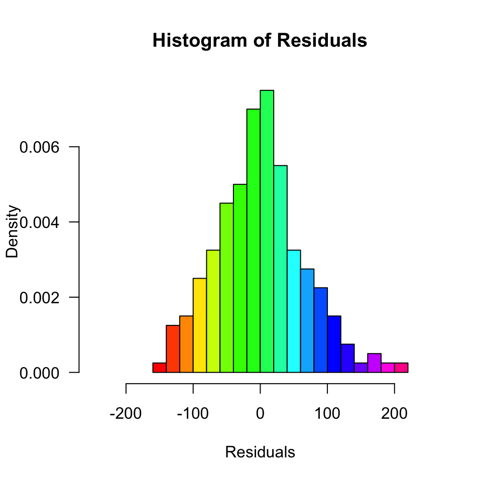
Normality of Residuals
Are the residuals normally distributed?
Model fit
- The fit of the model can be viewed in terms of the correlation (\(r\)) between the predictions and the observed values: if the predictions are perfect, the correlation will be 1.
- For simple regression, this is equal to the correlation between adverts and sales. For multiple regression (block 3), these will differ.
r <- cor(prediction, sales)
r
[1] 0.5784877Explained variance
Squaring this correlation gives the proportion of variance in sales that is explained by adverts:
r^2[1] 0.3346481Explained variance visually (\(n = 10\))
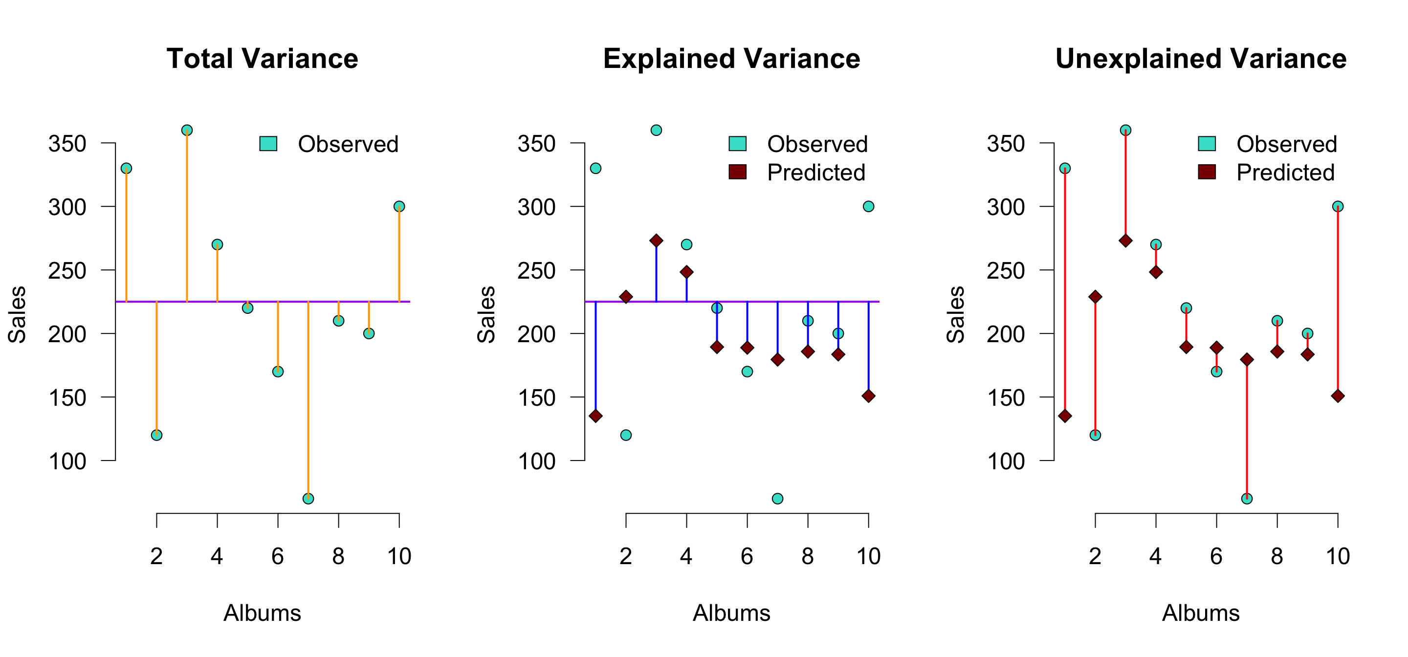
\(r^2\) is the proportion of blue to orange, while \(1 - r^2\) is the proportion of red to orange
Calculate t-values for b’s for hypothesis testing
We can also convert the slope \(b_1\) to a \(t\)-statistic, since that has a known sampling distribution:
\[\begin{aligned} t_{n-p-1} &= \frac{b_1 - \mu_{b_1}}{{SE}_{b_1}} \\ df &= n - p - 1 \\ \end{aligned}\]
Where \(b_1\) is the beta coefficient, \({SE}\) is the standard error of the beta coefficient, \(n\) is the number of subjects and \(p\) the number of predictors. \(\mu_{b_1}\) is the null-hypothesized value for \(b_1\) - usually set to 0.
Converting b to \(t\)
# Get Standard error's for b (bonus)
se.b1 <- sqrt((n/(n-2)) * mean(error^2) / (var(adverts) * (n-1))); se.b1
[1] 0.009632366# Calculate t for b1
mu.b1 <- 0
t.b1 <- (b1 - mu.b1) / se.b1; t.b1[1] 9.979322n <- nrow(data) # number of rows
p <- 1 # number of predictors
df.b1 <- n - p - 1\(p\)-value for \(b_1\)
Locate in \(t\)-distribution
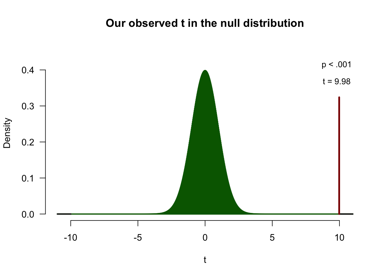
\[P(|t| \geq 9.98 \mid H_0) < .001\]
So how many @!&#$ ways do we have for assessing an association?!
# the correlation between x and y, standardized (between -1, 1)
cor(sales, adverts)    # .58: moderate and positive, whatever the units were
[1] 0.5784877# the covariance between x and y, unstandardized
cov(sales, adverts) # same association but original units[1] 22672.02# regression coefficient in linear regression, unstandardized
# generalizes easily to settings with multiple predictors
b1 # how much does y-prediction increase, if we increase x by 1 unit?[1] 0.09612449# t-statistic: standardized difference between b1 and 0
t.b1 # used for testing the null hypothesis that b1 = 0[1] 9.979322 # 9.98: b1 sits about ten standard errors above zero
# The metrics below are more indicative of an overall model's performance
# the correlation between y and model prediction, standardized (between -1, 1)
cor(sales, prediction) # can be squared to get proportion explained variance[1] 0.5784877 # same as original cor: one predictor *is* the model
# squared -> .33, a third of the variance in sales
# is explained by advertisingMove \(r\), \(s_x\) and \(s_y\) around and watch the covariance, the slope and \(r\) respond
Closing
Exam note
Alternative hypothesis:
- The question context tells you which test/alternative hypothesis to use
- Linear regression in JASP only reports two-sided \(p\), so those stay two-sided
Assumptions:
- Only assessing the assumptions, not yet how to handle violations
- Only Sensitivity (scatterplot, casewise diagnostics), Normality (Q-Q plot), Linearity (scatterplot, residuals vs. predicted)
- Don’t need to study ch6; lecture and application in ch8 suffice
See trial exam questions for examples of both
Next Week
- Exam!
- Mix of using JASP/interpreting output/conceptual understanding
- WA will have trial exam with old exam questions
- Field book available (like in the trial exam), including glossary
Recommended Exercises
Contact
